Classical Models in Epidemics¶

The classical models in epidemics are compartment models. In such models, the hosts are arranged into different populations such as susceptible populations, infected populations, and recovered populations.

SIR¶

Fig. 31 SIR model

The Kermack-McKendrick deterministic model describes the transitions between the different populations. The susceptible population \(S(t)\) decrease at a rate \(-\alpha I(t) S(t)\), where \(\beta\) is the average probability of getting infected by the infected population. The recovery rate of the infected population is \(\alpha\).

(48)¶\[\begin{split}\frac{dS(t)}{dt} &= -\beta I(t) S(t) \\ \frac{dI(t)}{dt} &= \beta S(t) I(t) - \alpha I(t),\end{split}\]

with the constraint

\[S(t) + I(t) + R(t) = N,\]

where \(N\) is the total population. [Martcheva2015]

The limiting behavior of the system is also intuitive. If the infected population is quarantined, i.e., \(\beta=0\), the infected population decays exponentially with a half-life \(1/\alpha\). Notice that the populations can only be integers. When \(S(t)<1\), the infected population moves to the exponential decay phase.

At a specific time \(t=t_t\), we might reach the threshold that

\[\beta S(t_t) - \alpha = 0.\]

Suppose the susceptible population is larger initially, we would have \(\beta S(t_0) - \alpha > 0\) initially. The infected population will grow. The threshold indicates a flipping moment when the infected population will start to decrease.

The threshold requires

\[\frac{\beta S(t_t)}{\alpha} = 1.\]

When \(\frac{\beta S(t_t)}{\alpha}>1\), the infected population is growing. It is convinient to define

\[\tau(t) = \frac{\beta S(t)}{\alpha},\]

with which equations (48) becomes

\[\begin{split}\frac{dS(t)}{dt} &= - \alpha \tau(t) I(t) \\ \frac{dI(t)}{dt} &= \alpha (\tau(t) - 1) I(t),\end{split}\]

If \(\tau(t)>1\), the infected population will grow. If \(\tau(t)<1\), the infected population will decrease.

In the very beginning of a epidemic event, the susceptible population fraction is almost constant, thus \(\tau(t)\) is almost constant, i.e., \(\tau(t) = \tau_0\), the growth rate of \(I(t)\) is

\[\frac{dI(t)}{dt} = \alpha (\tau_0 - 1) I(t).\]

The equations are solved

\[I(t) = I(t_0) e^{\alpha (\tau_0 - 1) t}.\]

The exponential growth rate is determined by

\[\alpha (\tau_0 - 1).\]

The days \(\Delta t\) required to double the infected population is a constant in the early stage. To find out \(\Delta t_d\),

\[\frac{I(t+\Delta t)}{I(t)} = e^{\alpha (\tau_0 - 1) \Delta t} \equiv 2,\]

which leads to

\[\Delta t = \frac{\ln 2}{\alpha(\tau_0 -1)} \sim \frac{0.7}{\alpha(\tau_0 -1)} .\]

Simulate SIR Using Poisson Process¶

The transition events of a susceptible person being infected (\(S\to I\)) and an infected person being recovered (\(I\to R\)).

The rates are determined by the equation (48),

\[Y_{S\to I}\left(\int_0^t \beta I(t') S(t') dt' \right)\]

and

\[Y_{I\to R}\left( \int_0^t \alpha I(t') dt' \right).\]

Whenever an event is triggered in the process \(Y_{S\to I}\), we will have one more infected person and one less susceptible person.

In fact, \(1/\alpha\) is the mean days an infected person remains in the infectd status. This is used to estimate the \(\alpha\) using data. The value of \(\beta\) is estimated using the relation [Martcheva2015]

\[\frac{\beta}{\alpha} = \frac{\ln (S(t_0)/S(t\to\infty))}{S(t_0) + I(t_0) - S(t\to\infty) }\]

SIS¶

Some epidemics such as influenza infect us repeatedly. One simple model for them is the SIS model shown in figure SIS model.,

Fig. 32 SIS model.

The dynamics are determined by

\[\frac{dI(t)}{dt} = \beta I(t) S(t) - \alpha I(t),\]

with the constraint

\[S(t) + I(t) = N.\]

The dynamics of the basic SIS model is determined by one single first-order differential equation

\[\begin{split}\frac{dI(t)}{dt} &= \beta I(t) (N - I(t)) - \alpha I(t) \\ &= (\beta N - \alpha )I(t) - \beta I(t) I(t) \\ &= (\beta N - \alpha )I(t) \left( 1 - \frac{I(t)}{(\beta N - \alpha)/\beta} \right) \\ &\equiv r \left(1 - \frac{I}{r/\beta}\right) I(t),\end{split}\]

where we defined the growth rate

\[r \equiv \beta N - \alpha = \alpha(\frac{\beta}{\alpha} N - 1) \equiv \alpha (\mathscr R_0 - 1).\]

The parameter \(\mathscr R_0\) is the basic reproduction number,

\[\mathscr R_0 = \frac{\beta}{\alpha} N .\]

If \(\mathscr R_0 > 1\), we get a positive growth grate for \(I(t)\). Otherwise, the infected population will decrease.

Basic Reproduction Rate

A quote from the Martcheva [Martcheva2015]

Epidemiologically, the reproduction number gives the number of secondary cases one infectious individual will produce in a population consisting only of susceptible individuals.

Vector-Borne¶

Some diseases are transmitted from one host to another with some intermediate living carriers such as arthropod. An intermediate living carrier is called a vector. Vectors do not get sick because of the pathogenic microorganism but they will carry the pathogenic microorganism throughout their lives.

To model the vector-borne diseases, two populations are added to the model, the infected population of vectors \(I_v(t)\) and the susceptible population of vectors \(S_v(t)\). Apart from being infected by the infected hosts, the birth rate \(\Lambda_v\) and the death rate \(\mu\) of the vectors are also related to the two populations. Thus the two populations are coupled to the different populations of the hosts,

\[\begin{split}\frac{S_v(t)}{dt} &= \Lambda_v - p a S_v(t) I(t) -\mu S_v(t) \\ \frac{I_v(t)}{dt} &= p a S_v(t) I(t) - \mu I_v,\end{split}\]

where \(a\) is the rate of a vector biting a host, \(p\) is the rate of a vector being infected when biting an infected host. The product \(pa\) is the rate of a vector being infected. [Martcheva2015]

Because most vector-borne diseases are repeatative, we combine the dynamics of the vectors with the SIS model with the constraint \(S(t) + I(t) = N\),

\[\frac{I(t)}{dt} = qa S(t) I_v(t) -\alpha I(t),\]

where \(q\) is the rate of being transmitted from the vector to the host, \(\alpha\) is the recovery rate. The recovered hosts become susceptible.

Generalization¶

A general compartment model is a model may include other stages of the disease. The differential equations are easily translated from the flowcharts.

In the disease progression, four stages are relevant. [Martcheva2015]

Exposed stage E or latent stage L: infected but not infectious;
Asymptomatic stage A: the asymptomatic stage describes the asymptomatic infection or subclinical infection where the host is infected by no symptoms are shown;
Carrier stage C: infected but not sick;
Passive immunity stage M: antibodies are transferred between hosts.

Fig. 33 SEIR model

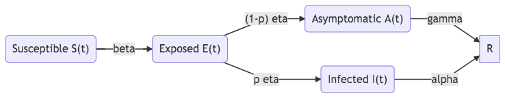
Fig. 34 SEIR model with an asymptomatic stage

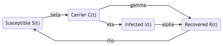
Fig. 35 SCIRS model

Compartments related to epidemic control can also be integrated into the models.

Quarantine Q
Treatment T
Vaccination V

Fig. 36 SIQR model

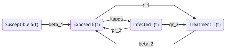
Fig. 37 SEIT model

Each compartment is also subject to variants based on the demographics of the populations, heterogeneities of the pathogens and hosts. [Martcheva2015]

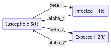
Fig. 38 SIS with two strains

Basic Reproduction Number and Stability Analysis¶

Consider the SIR model (48) and add birth rate \(\Lambda\) and death rate \(\mu\) to the model,

\[\begin{split}\frac{dS(t)}{dt} &= \Lambda - \beta I(t) S(t) - \mu S(t)\\ \frac{dI(t)}{dt} & = \beta I(t) S(t) - \alpha I(t) - \mu I(t) \\ \frac{dN(t)}{dt} &= \alpha I(t) - \mu N(t),\end{split}\]

with

\[R(t) + I(t) + S(t) = N(t).\]

The reproduction number is

\[\mathscr R_0 = \frac{\Lambda \beta}{\mu(\alpha + \mu)}.\]

Since the equation for \(N(t)\) is independent of \(S(t)\) and \(I(t)\), the stability is determined by the first two equations. Denote the equilibrium point as \(S_0, I_0\), we linearize the equations using Linear Stability Analysis and find that the characteristic equation is related to \(\mathscr R_0\), i.e., the growth rate of the linearized system \(\lambda\) is a function of \(\mathscr R_0\) thus the stability of the system is also related to the reproduction number. Though the compartment model can be complicated as more stages are added, linear stability analysis is a very effective tool to analyze the stability.

References¶

[Martcheva2015]

(1, 2, 3, 4, 5, 6) Martcheva, M. (2015). Introduction to Epidemic Modeling, 9–31.

[Hill2016]

Learning Scientific Programming with Python