Equilibrium Statistical Mechanics Summary
Note
This is a review of equilibrium statistical mechanics. Though I called it a review, it is more like a list of keywords at this moment.
Review of Thermodynamics
Description of States in statistical mechanmics: thermodynamical quantities as macroscopic state;
Kinematics: equation of state; Thermodynamic Potentials.

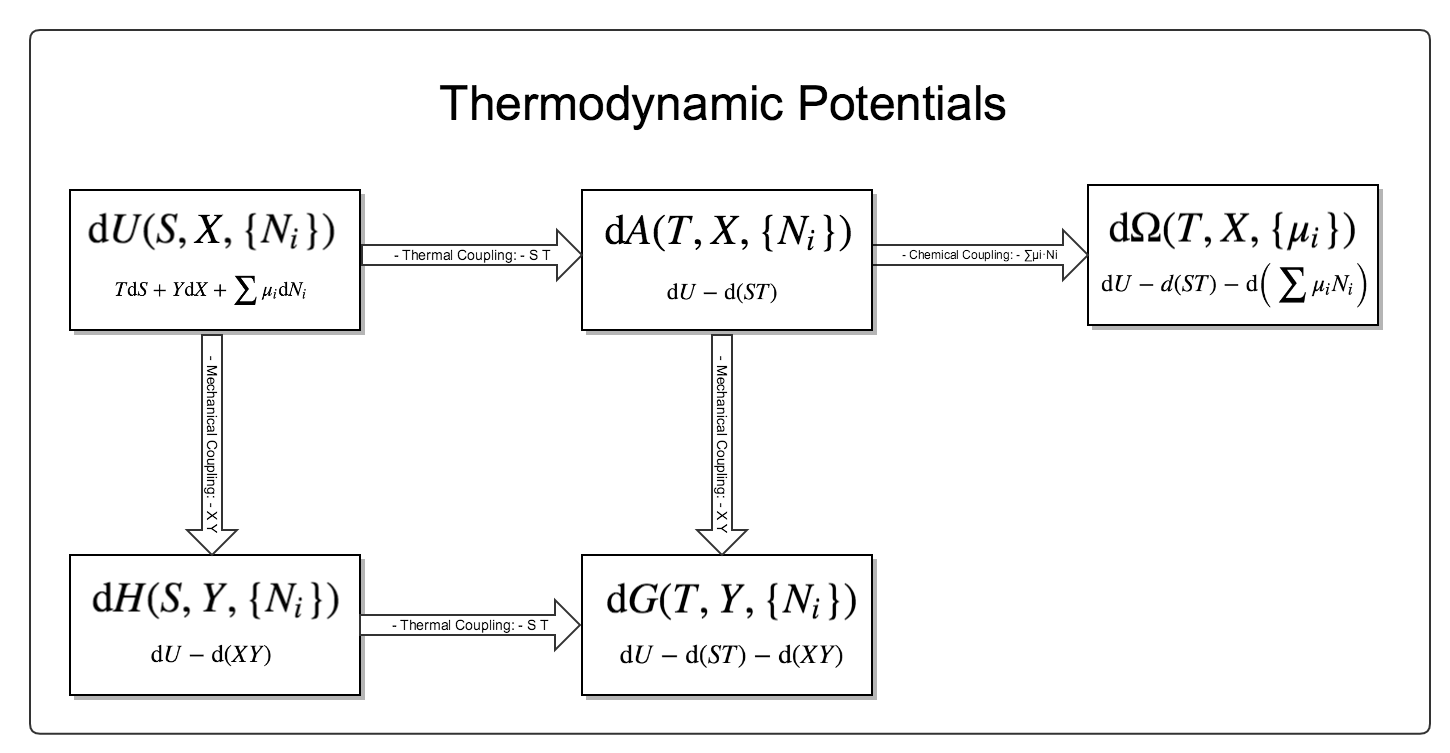
Fig. 6 The relationship between different thermodynamic potentials. There are three different couplings and five different potentials. For more details please read vocabulary Thermodynamic Potentials .
First principles: The Laws of Four
Dynamics: Phase transition; Stability; Response
Description of the Microstates
For a system with \(N\) particles of \(r\) degrees of freedom, we could always describe the microstates of the system by looking at the state of each particle. There are at least two different point of views, the \(\mu\) space (mu space) and the \(\Gamma\) space (Gamma space).
The \(\mu\) space is a \(r\) dimensional space where each dimension corresponds to one degree of freedom of the particle. Thus a point in the \(\mu\) space represents a the state of one particle. To represent the microstate of the whole system, we need \(N\) points in the \(\mu\) space.
The \(\Gamma\) space is a \(rN\) dimensional space. In the \(\Gamma\) space, we have a holistic view. Each point in the \(\Gamma\) space represents the state of all the particles. For example, we use the first \(r\) dimensions out of the \(rN\) dimension to represent the state of the first particle, the next \(r\) dimensions to represent the state of the second particle, and so on.
Why Distingushing between Microstates and Macrostates
In physical systems, we observe limited quantities regarding the internal structure. If we take the Bayesian point of view, we have the freedom to choose the amount of information we would like to use as priors. In statistical mechanics, macrostates is related to our view of the priors.
What is Statistical Mechanics
Physical systems are usually composed of a large amount of particles. In principle, we could calculate the observable quantities if we know the exact motions of the particles. For example, we only need the momentum transfer per unit area to know the pressure of the gas and momentum transfer could be calculated if we know the motion of the particles.
This method is obviously unrealistic given the number of particles that we are dealing with. Alternatively, we could figure out the probabilities of each possible values of the observable quantities, i.e., the probability of the system being on each point in the \(\Gamma\) space. For each microscopic state, we could calculate the thermodynamic observables corresponding to it.
However, this approach requires a first principle that we could use to figure out the distribution of the observables \(\{\mathscr O_i\}\), i.e., \(p(\{\mathscr O_i\})\). More regoriously, it is expected that we derive a theory that tells us the conditional probability \(p(\{\mathscr O_i\} \vert t, \{m_i, r_i\})\) where \(\{m_i, r_i\}\) is a set of features that are defined by the materials, the enviroment and the restrictions, \(t\) is time.
A Bayesian View
In Bayesian statistics,
\(p(\{\mathscr O_i\})\) is the prior distribution and is observed in experiments.
Ideally, it would be a perfect model if we determine the joint distribution \(p(\{\mathscr O_i\}, \{m_i, r_i\})\). The marginalized distribution \(p(\{\mathscr O_i\}) = \int p(\{\mathscr O_i\}, \{m_i, r_i\}) \mathrm d\{m_i, r_i\}\) corresponds to our observations. This joint distribution connects the microscopic view and the macroscopic view. However, it is utterly impossible to calculate the details of the probabilities for areal-world statistical system. First, we have no information of the initial state. We have to introduce the stochastic processes to describe the states. Secondly, this joint probability often becomes very hard to compute when we introduce interactions between the particles.
Nevertheless, we can still perform some analysis using approximations. If we ask for the probability of the microscopic states for given macroscopic observables, we have the inference
where \(p(\{\mathscr O_i\} \mid \{m_i, r_i\})\) is given by a physics model such as momentum transfer as pressure of ideal gas, \(p(\{m_i, r_i\}\) is given by some prior knowledge such as Boltzmann’s equal a priori probability, \(p(\{\mathscr O_i\})\) is from observation.
Computation aside, this formalism brings in the question of how our statistical theory of matter can be validated. There are two sides in the theory: A statistical model that predicts the most prominent values of the observables as well as the confidence, and the sampled probability distributions of observables from our experiments. To validate the statistical model, we perform some kind of hypothesis test.
On the other hand, real-world statistical physics deals with a huge amount of particles which leads to an extremely narrow confidence interval. We can simply match the results without considering the fluctuations.
For example, the Boltzmann theory assume equal a priori probabilities for the microstates. In Boltzmann theory, we need two aspects of knowledge to understand the statistical system.
- The distribution of the mirostates, which has been assumed to be equal.
- How the energy of combinations of single particles are calculated. For example, this refers to the calculation of the energy levels in quantum mechanics.
The Two Approaches of Statistical Mechanics
The probability distribution of the microscopic states of the system, \(p(\{O_i\})\), is needed to estimate the observables \(\{O_i\}\). For example, to estimate the energy of the system, we take the statistical average using the distribution \(\int E p(E) \mathrm dE\).
However the microscopic state of the system is not known in general. We have to apply some assumptions and tricks.
There are two famous approaches developed in statistical mechanics. The Boltzmann’s approach is utilizing the most probable distributions while the Gibbs’ approach is using ensembles. They do not only differ from the way of estimating the probabilities of the states but also differ philosophically.

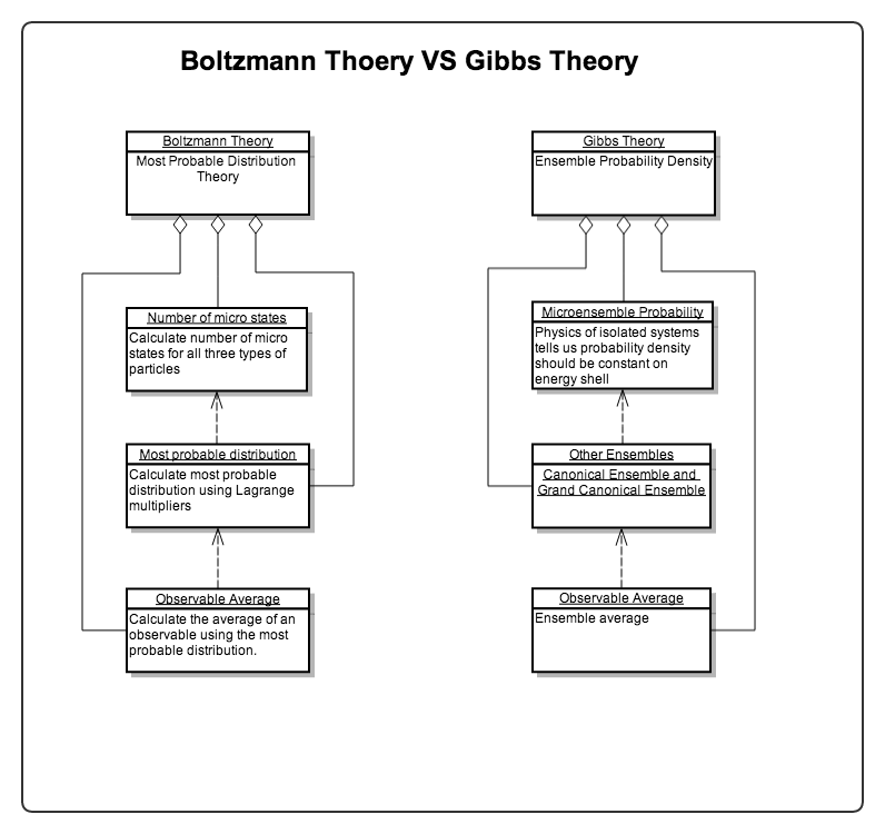
Fig. 7 Modeling of the two theories. Refer to Most Probable Distribution.
Boltzmann Statistics
As mentioned in Description of the Microstates, many microstates have the same observables such as energy \(E\). For each value of energy, we could figure out the number of microstates, the distribution of microstates \(\Omega(E, \cdots)\). What makes this distribution powerful is that we could figure out the total number of microstates for this distribution by integrating or summing up for all energies \(\int \Omega(E, \cdots) \mathrm d E \mathrm d\cdots\). The total number of microstates is closely related the the probability of this distribution as will be discussed below. Meanwhile, we could calculate the thermodynamic observables using the distribution.
In statistical physics, we will be focusing on the distribution of the microstates with respect to thermodynamic variables.
In Boltzmann statistics, we follow these guidelines.
- Two postulates:
- Occurrence of state in phase space ( Equal A Prior Probability ): all microstates have the same probabilities of occurence; This means that the most probable distribution for different energy \(\Omega(E, \cdots)\) should have the largest total number of microstates, \(\int \Omega(E, \cdots) \mathrm d E \mathrm d\cdots\).
- The most probable energy state is the state that an equilibrium system is staying at. This means that the most probable distribution discussed in 1 will be the actual distribution of the system. This postulate is not precise but there is a reason why it works. The distribution of the energy states is an extremely sharp peak at the most probable state.
- We find the most probable distrinution by maximizing the total number of microstates. Boltzmann distribution and Boltzmann factor is derived from this.
- Partition function makes it easy to calculate the observables.
- Density of state \(g(E)\) ;
- Partition function \(Z = \int g(E) \exp(-\beta E) \mathrm dE\); Variable of integration can be changed;
- Systems of 3N DoFs \(Z = Z_1^{3N}\).
- Macroscopic observables are calculated by taking specific transformations such as derivatives of the partition function.
- Observable
- Assumptions about free energy \(A = - k_B T\ln Z\); Combine this with thermodynamics potential relations we can calculate entropy then everything.
- Internal energy \(U = \avg{E} = - \partial_\beta \ln Z\); All quantities can be extracted from partition function except those serve as variables of internal energy.
- Heat capacity \(C = \partial_T U\)
Gibbs Ensemble Theory
- Ensembles
- Density of states; Liouville equation; Von Neumann equation
- Equilibrium
- Three ensembles
- Observables
Boltzmann Factor
Boltzmann factor appears many times in thermodynamics and statistical mechanics. In Boltzmann’s most probable theory, ensemble theory, etc.
Applications of These Theories
Oscillators
Theories of chains of oscillators in different dimensions are very useful. In fact the fun thing is, most of the analytically solvable models in physics are harmonic oscillators.
A nice practice for this kind of problem is to calculate the heat capacity of diatom chain. A chain of N atom with alternating mass M and m interacting only through nearest neighbors.
The plan for this problem is
- Write down the equation of motion for the whole system;
- Fourier transform the system to decouple the modes (by finding the eigen modes);
- Solve the eigen modes;
- Calculate the partition function of each mode;
- Sum over each mode.
Problem is, we usually can not solve the problem exactly. So we turn to Debye theory. Debye theory assumes continuous spectrum even though our boundary condition quantizes the spectrum. So we need to turn the summation into integration using DoS using any of the several ways of obtaining DoS. Finally we analyze the different limits to get the low temperature or high temperature behavior.
Hint
Here are several methods to obtain DoS. To do!
Heat Capacity
- Classical theory: equipartition theorem;
- Einstein theory: all modes of oscillations are the same;
- Debye theory: difference between modes of oscillations are considered.
Gibbs Mixing Paradox
Gibbs Mixing Paradox is important for the coming in of quantum statistical mechanics.
Mean Field Theory
Mean Field Thoery is the idea of treating interaction between particles as interactions between particles and a mean field.
Van der Waals Gas
Van der Waals Gas can be derived using Mayer expansion and Leonard-Jones potential.