A More Systematic View¶

Ensemble¶

A standard procedure of solving mechanics problems is

Initial condition / Description of states -> Time evolution -> Extraction of observables

States¶

Density of states in phase space

Continuity equation

\[\partial _ t \rho + \nabla \cdot (\rho \vec u) =0\]

This conservation law can be more simpler if dropped the term \(\nabla\cdot \vec u = 0\) for incompressibility.

Or more generally,

\[\partial _ t \rho + \nabla \cdot \vec j = 0\]

and here \(\vec j\) can take other definitions like \(\vec j = - D \partial_x \rho\).

This second continuity equation can represent any conservation law provided the proper \(\vec j\).

From continuity equation to Liouville theorem

From continuity equation to Liouville theorem:

We start from

\[\frac{\partial}{\partial t} \rho + \vec \nabla \cdot (\rho \vec v)\]

Divergence means

\[\vec \nabla \cdot = \sum_i \left( \frac{\partial}{\partial q_i} + \frac{\partial}{\partial p_i} \right) .\]

Then we will have the initial expression written as

\[\frac{\partial}{\partial t} \rho + \sum_i \left( \frac{\partial}{\partial q_i} (\rho \dot q_i) + \frac{\partial}{\partial \dot p_i} \right) .\]

Expand the derivatives,

\[\frac{\partial}{\partial t} \rho + \sum_i \left[ \left( \frac{\partial}{\partial q_i} \dot q_i + \frac{\partial}{\partial p_i} \dot p_i\right) \rho + \dot q_i \frac{\partial}{\partial q_i} \rho + \dot p_i \frac{\partial}{\partial p_i} \rho \right] .\]

Recall that Hamiltonian equations

\[ \begin{align}\begin{aligned}\dot q_i = \frac{\partial H}{\partial p_i}\\\dot p_i = - \frac{\partial H}{\partial q_i}\end{aligned}\end{align} \]

Then

\[\left( \frac{\partial}{\partial q_i} \dot q_i + \frac{\partial}{\partial p_i} \dot p_i\right) \rho .\]

Finally convective time derivative becomes zero because \(\rho\) is not changing with time in a comoving frame like perfect fluid.

\[\frac{d}{d t} \rho \equiv \frac{\partial}{\partial t}\rho + \sum_i \left[ \dot q_i \frac{\partial}{\partial q_i} \rho + \dot p_i \frac{\partial}{\partial p_i} \rho \right] =0\]

Time evolution¶

Apply Hamiltonian dynamics to this continuity equation, we can get

\[\partial_t \rho = \{H, \rho\}\]

which is very similar to quantum density matrix operator

\[\mathrm i \hbar \partial_t \hat \rho = [ \hat H, \hat \rho ]\]

That is to say, the time evolution is solved if we can find out the Poisson bracket of Hamiltonian and probability density.

Requirements for Liouville Density¶

Liouville theorem;
Normalizable;

Hint

What about a system with constant probability for each state all over the phase space? This is not normalizable. Such a system can not really pick out a value. It seems that the probability to be on states with a constant energy is zero. So no such system really exist. I guess?

Like this?

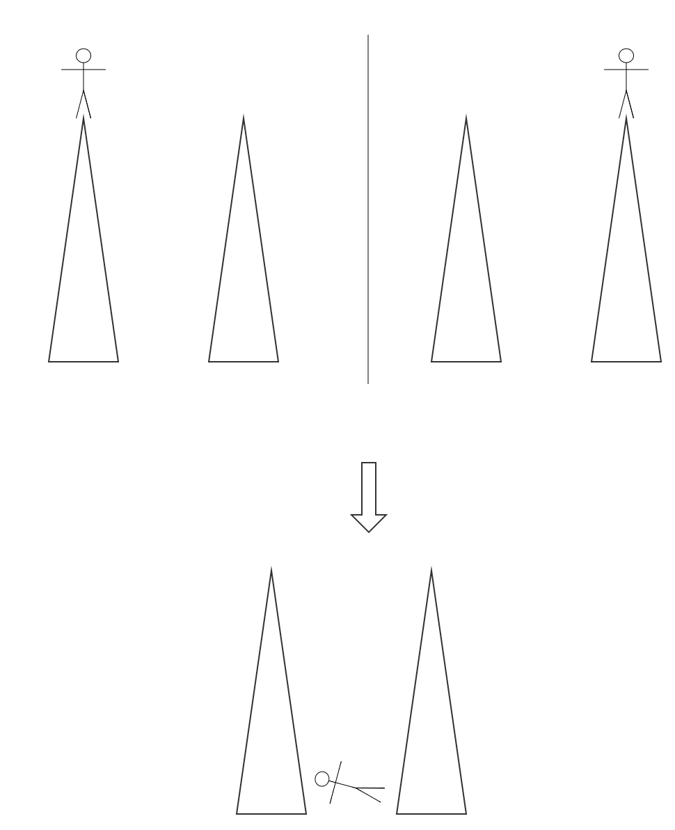
Someone have 50% probability each to stop on one of the two Sandia Peaks for a picnic. Can we do an average for such a system? Example by Professor Kenkre.

And one more for equilibrium systems, \(\partial_t \rho =0\).

Extraction of observables¶

It’s simply done by calculating the ensemble average

\[\langle O \rangle = \int O(p_i; q_i;t) \rho(p_i;q_i;t) \sum_i dp_i dq_i dt\]

where \(i=1,2,..., 3N\).