Quantum Master Equation
.._Quantum Master Equation:
Quantum Master Equation
Density Matrix
In quantum mechanics, the probability doesn’t deliver all the information available. The density matrix is a better choice to construct a master equation for quantum systems.
Quantum mechanics observables are averages over all the density matrix elements,
\[\langle O \rangle = \sum_{m,n} O_{nm}\rho_{mn}.\]
Given an initial condition with diagonalized density matrix, the dynamics won’t necessarily guarantee the diagonalizion of the density matrix. Thus the average pickup off-diagonal element contributions as time goes on.
The classical master equations won’t solve authentic quantum problems given the different definition of the average of the observables.
To derive a quantum master equation, we start from the first principle in quantum mechanics,
\[i\hbar \frac{d}{dt}\hat \rho = [\hat H,\hat \rho] \equiv \hat L \hat \rho.\]
Pauli’s Mistake
Pauli derived the first quantum master equation. However, it was not quite right.
The formal solution to a quantum system is
\[\hat \rho(t) = e^{-iL(t-t_0)} \hat \rho(t_0) .\]
In the Heisenberg picture,
\[\hat \rho(t+\tau) = e^{-i\tau \hat H} \hat \rho(t) e^{i\tau \hat H} .\]
The diagonal elements of the density matrix are
\[\rho_{mm}(t+\tau) = \bra{m}e^{-i\tau \hat H} \hat \rho(t) e^{i\tau \hat H} \ket{m}.\]
On the left hand side, \(P_m\equiv \rho_{mm}\) is the probability of the state. The right hand side becomes
\[\text{RHS} = \sum_{n,l}\bra{m}e^{-i\tau \hat H} \ket{n} \bra{n}\hat \rho(t) \ket{l}\bra{l} e^{i\tau \hat H} \ket{m}.\]
Pauli’s then assumed that the system is “dirty” enought to have recurances of diagonalized density matrix. The diagonalized density matrix is used to calculate the probability,
\[\begin{split}P_m(t+\tau) &= \sum_{n}\bra{m}e^{-i\tau \hat H} \ket{n} \bra{n}\hat \rho(t) \ket{n}\bra{n} e^{i\tau \hat H} \ket{m} \\
& = \sum_{n} P_n \left\vert \bra{m} e^{-i\tau \hat H} \ket{n} \right\vert^2 .\end{split}\]
The term \(\left\vert \bra{m} e^{-i\tau \hat H} \ket{n} \right\vert^2\) on the right hand side is the transition probability from a state n to state m in a short period \(\tau\). We define
\[Q_{mn}(\tau) \equiv \left\vert \bra{m} e^{-i\tau \hat H} \ket{n} \right\vert^2.\]
The probability at time \(t+\tau\) is
\[P_m(t+\tau) = \sum_n Q_{mn}(\tau)P_n(t).\]
The Chapman method is applied to derive the master eqution.
Fermi’s Golden Rule
The Pauli assumption is the Fermi golden rule which requires an infinite amount of time. This is not gererally valid.
Better Quantum Master Equations
The first “real” quantum master equation was derived by van Hove.
van Hove argued that Pauli’s result is not correct. First of all,
\[\begin{split}P_m(t+\tau) &= \sum_n Q_{mn}(\tau) P_n(t) \\
P_m(t-\tau) & = \sum_n Q_{mn}(-\tau) P_n(t) .\end{split}\]
With \(Q_{mn}(\tau) = Q_{mn}(-\tau)\), we have
\[\begin{split}Q_{mn}(\tau) & = \left\vert \bra{m} e^{-i\tau \hat H} \ket{n} \right\vert^2 \\
& = \left\vert \bra{m} e^{i\tau \hat H} \ket{n} \right\vert^2 \\
& = Q_{mn}(-\tau),\end{split}\]
which leads to
\[P_m(t+\tau) = P_m(t-\tau).\]
In other words, we’ve shown that the probabilities of states are constant.
van Hove
Questions
There are several key questions in inventing a quantum master equation.
- Which systems can be described by the master equations?
- What’s the time scale for quantum master equation to be valid?
Suppose we have a quantum system with the Hamiltonian
\[\hat H = \hat H_0 + \lambda(t)\hat W .\]
van Hove’s method was to describe systems with diagonal singularity conditions on a large time scale. The perturbations should be small enough, i.e., \(\lambda^2 t \approx \text{constant}\). The diagonal elements are
(37)\[\begin{split}P_m & = \bra{m}\hat \rho \ket{m} \\
& = \sum_{m,n} \bra{m} e^{i\hat H t/\hbar} \ket{n}\bra{n} \hat \rho(0) \ket{l}\bra{l} e^{-iHt/\hbar} \ket{m} \\
& = \sum_{m,n} \left\vert \bra{m} e^{i (\hat H_0 + \lambda \hat W) t/\hbar } \ket{n} \right\vert^2 \rho_{nl}(0) .\end{split}\]
van Hove applied random phase condition on the initial condition, i.e., \(\rho_{nl}(0)\) is diagonalized at initial \(t=0\). We have
\[\rho_{nl} (0) = \rho_{nn} \delta_{nl} = P_n(0) \delta_{nl},\]
Equation (37) becomes,
(38)\[P_m = \sum_n \left\vert \bra{m} e^{i (\hat H_0 + \lambda \hat W) t/\hbar } \ket{n} \right\vert^2 P_n(0) .\]
The equation (38) is furthure simplified by the Dyson series.
Zwawzig and Nakajiwa
Zwawzig and Nakajiwa invented the projection technique to solve quantum master equations.
We define a diagonalizing operator \(\hat D\) which keeps the diagonal elements and drops the off-diagonal elements of a matrix. With this definition, it’s conjugate \(1-\hat D\) will drop all diagonal elements.
The diagonalized density matrix is
\[\hat \rho_d = \hat D \hat \rho\]
and the all the off-diagonal elements of the density matrix
\[\hat \rho_{od} = (1-\hat D)\hat \rho.\]
Reconstruct the Density Matrix
The density matrix is trivilly reconstructed by
\[\hat \rho = \hat \rho_d + \hat \rho_{od} .\]
The von Neumann equation is
\[i\hbar \partial_t \hat \rho = \left[\hat H, \hat \rho \right],\]
With the Liouville operator \(\hat L\), the von Neumann equation is rewritten as
\[\partial_t \hat \rho = -i \hat L \hat \rho .\]
Apply \(\hat D\) and \(1-\hat D\) to the von Neumann equation, we get two equations
(39)\[\begin{split}\partial_t \hat \rho_d & = -i \hat D \hat L \hat \rho \\
\partial_t \hat \rho _{od} & = -i (1 - \hat D) \hat L \hat \rho .\end{split}\]
Use the completeness relation \(\hat \rho = \hat \rho_d + \hat \rho_{od}\),
(40)\[\begin{split}\partial_t \hat \rho_d & = -i \hat D \hat L \hat \rho_d - i \hat D \hat L \hat \rho _ {od} \\
\partial_t \hat \rho _{od} & = - i (1 - \hat D) \hat L \hat \rho _ d - i (1 - \hat D) \hat L \hat \rho_{od} .\end{split}\]
The off-diagonal equation in equation (40) is solved using Green’s function,
(41)\[\hat \rho_{od} = e^{-i(1-\hat D)\hat L t} + \int_0^t dt' e^{-i(1-\hat D) \hat L (t-t')}(-i(1-\hat D)\hat L \hat \rho_d(t')) .\]
Green’s Function
Recall that the solution to
\[\dot y + \alpha y = f\]
is
\[y = e^{-\alpha t} y(0) + \int_0^t dt' e^{-\alpha (t-t')} f(t') .\]
Insert (41) into the equation for \(\hat \rho_d\) in equation (40),
(42)\[{\color{red}\partial_t \hat \rho_d = - i\hat D\hat L \hat \rho_d - \hat D\hat L \int_0^t dt' e^{-i(1-\hat D) \hat L (t-t')}(1-\hat D)\hat L \hat \rho_d(t')} {\color{blue} - i \hat D \hat L e^{-i(1-\hat D)\hat L t} \rho_{od}(0) }.\]
The term \(- i \hat D \hat L e^{-i(1-\hat D)\hat L t} \rho_{od}(0)\) disapears when we apply the random phase initial condition. Then we get our closed master equation for \(\hat \rho_d\), i.e., an equation for the probabilities,
(43)\[{\color{red}\partial_t \hat \rho_d = - i\hat D\hat L \hat \rho_d - \hat D\hat L \int_0^t dt' e^{-i(1-\hat D) \hat L (t-t')}(1-\hat D)\hat L \hat \rho_d(t')}.\]
The Off-diagonal Elements
“We can always use phasers.”
—V. M. Kenkre
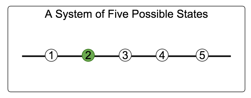
The condition \(\rho_{od}(0)=0\) needed to reach a closed master equation doens’t imply that we have to require localized initial condition on any specific state.
Given a system of five possible states, the off-diagonal elements are zeros if the system is on a specific state initially.
The density matrix might contain off-diagonal elements if we have two non-orthogonal states initially.
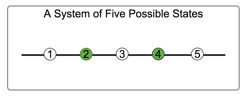
However, we can always choose a combination of the current basis to diagonalize the density matrix.
The projection technique can also be applied on the flavor transformations of neutrinos.
Simplify the Quantum Master Equation
We derived the quantum master equation using the projection method. However, the equation is complicated.
Let’s stare at the solution equation (43) for a minute,
\[{\color{red}\partial_t \hat \rho_d = - i\hat D\hat L \hat \rho_d - \hat D\hat L \int_0^t dt' e^{-i(1-\hat D) \hat L (t-t')}(1-\hat D)\hat L \hat \rho_d(t')} {\color{blue} - i \hat D \hat L e^{-i(1-\hat D)\hat L t} \rho_{od}(0) }.\]
By definition, \(\rho_d=\hat D\rho\). The term on the right hand side \(\hat D \hat L \rho_d\) is
\[\begin{split}\hat D \hat L \rho_d & = \hat D\hat L \hat D \hat \rho \\
& = \hat D \left[ {\color{magenta} \begin{pmatrix}\rho_{11} & 0 & 0 & \cdots \\ 0 & \rho_{22} & 0 & \cdots \\ 0 & 0 & \rho_{33} & \cdots \\ \vdots & \vdots & \vdots & \ddots \end{pmatrix} \begin{pmatrix} H_{11} & H_{12} & H_{13} & \cdots \\ H_{21} & H_{22} & H_{23} & \cdots \\ H_{31} & H_{32} & H_{33} & \cdots \\ \vdots & \vdots \vdots & & \ddots \end{pmatrix} } - {\color{green} \begin{pmatrix} H_{11} & H_{12} & H_{13} & \cdots \\ H_{21} & H_{22} & H_{23} & \cdots \\ H_{31} & H_{32} & H_{33} & \cdots \\ \vdots & \vdots \vdots & & \ddots \end{pmatrix} \begin{pmatrix} \rho_{11} & 0 & 0 & \cdots \\ 0 & \rho_{22} & 0 & \cdots \\ 0 & 0 & \rho_{33} & \cdots \\ \vdots & \vdots & \ddots & \cdots \end{pmatrix} } \right]\end{split}\]
The diagonal elements are the same for the two terms (the magenta term and the green term) in the braket so that all the diagonal elements are gone. Finally, we apply \(\hat D\) to the off-diagonalized matrix and get 0,
\[\hat D \hat L \rho_d = 0.\]
Thus the first term on the right hand side in equation (43) \(-i\hat D\hat L\hat \rho_d = 0\).
In quantum perturbation theory, the Hamiltonian is \(\hat H = \hat H_0 + \lambda \hat W\). The Liouville operator for this system has two parts,
\[\hat L = \hat L_0 + \lambda \hat L_W.\]
The master equation becomes
\[\begin{split}\partial_t \hat \rho_d & = - \int_0^t dt' \hat D (\hat L_0 + \lambda \hat L_W ) e^{-i(1-\hat D) (\hat L_0 + \lambda \hat L_W )(t-t')}(1-\hat D)\hat L \hat \rho_d \\
& = - \int_0^t dt' \hat D (\hat L_0 + \lambda \hat L_W ) e^{-i(1-\hat D) (\hat L_0 + \lambda \hat L_W ) (t-t')} (\hat L_0 + \lambda \hat L_W ) \hat \rho_d \\
& = - \int_0^t dt' \mathscr K(t-t') \hat \rho_d .\end{split}\]
under the initial condition
\[- i \hat D \hat L e^{-i(1-\hat D)\hat L t} \rho_{od}(0) = 0\]
and the proved relation
\[\hat D \hat L \rho_d = 0.\]
Define
\[\mathscr K(t-t') = \hat D (\hat L_0 + \lambda \hat L_W ) e^{-i(1-\hat D) (\hat L_0 + \lambda \hat L_W ) (t-t')} (\hat L_0 + \lambda \hat L_W ) .\]
In the weak coupling interaction limit, \(\lambda \rightarrow 0\),
\[\begin{split}\mathscr K(t-t') &= \hat D (\hat L_0 + \lambda \hat L_W ) e^{-i(1-\hat D) (\hat L_0 + \lambda \hat L_W ) (t-t')} (\hat L_0 + \lambda \hat L_W ) \\
&= \hat D (\hat L_0 + \lambda \hat L_W ) e^{-i(1-\hat D) \hat L_0 (t-t')} (\hat L_0 + \lambda \hat L_W ) \\
&= \hat D \hat L_0 e^{-i(1-\hat D) \hat L_0 (t-t')} \hat L_0 + \lambda \hat D \hat L_0 e^{-i(1-\hat D) \hat L_0 (t-t')} \hat L_W \\
\phantom{\mathscr K(t-t')} & \phantom{{} = } + \lambda \hat D \hat L_W e^{-i(1-\hat D) \hat L_0 (t-t')} \hat L_0 + \lambda^2 \hat D \hat L_W e^{-i(1-\hat D) \hat L_0 (t-t')} \hat L_W \\
&= \lambda^2 \hat D \hat L_W e^{-i(1-\hat D) \hat L_0 (t-t')} \hat L_W \\
&= \lambda^2 \hat D \hat L_W e^{-i\hat L_0 (t-t')} \hat L_W .\end{split}\]
Several terms of \(\lambda\) are dropped.
We will derive the Fermi’s golden rule. First, we have
(44)\[\bra{m} \partial_t \rho_d \ket{m} = -\lambda^2 \bra{m} \int_0^t dt' \hat L_W e^{-i(t-t')\hat L_0} \hat L_W \rho_d(t') \ket{m}.\]
A Useful Relation
Here is a useful relation,
\[\begin{split}e^{iA\hat L} \hat O & = \hat O + i A \hat L \hat O + \frac{(iA)^2}{2} \hat L \hat L \hat O + \cdots \\
& = \hat O + iA[\hat H, \hat O] + \frac{(iA)^2}{2} [\hat H, [\hat H,\hat O]] + \cdots \\
& = e^{iA\hat H}\hat O e^{-iA\hat H}.\end{split}\]
By definition, \(\hat L_W \hat \rho_d = \frac{1}{\hbar}[W, \rho_d]\). Define
\[\hat{\mathscr M} = e^{-i(t-t')\hat H_0}[\hat V,\hat \rho_d]e^{i(t-t')\hat H_0}.\]
Equation (44) becomes
(45)\[\begin{split}\bra{m} \partial_t \rho_d \ket{m} &= -\lambda^2 \bra{m} \int_0^t dt' [\hat W, e^{-i(t-t')\hat L_0}[\hat W, \rho_d(t')]] \ket{m} \\
& = -\lambda^2 \bra{m} \int_0^t [\hat W, ] dt' \ket{m} \\
& = -\lambda^2 \left( \bra{m} \int_0^t dt' \hat W\hat{\mathscr M} \ket{m} - \bra{m} \int_0^t \hat{\mathscr M}\hat W\ket{m} dt' \right) \\
& = -\lambda^2 \int_0^t dt' \left( \bra{m} \hat W\hat{\mathscr M} \ket{m} - \bra{m} \hat{\mathscr M}\hat W\ket{m} \right) \\
& = -\lambda^2 \int_0^t dt' \sum_n (W_{mn}\mathscr M_{nm} - \mathscr M_{mn}W_{nm}).\end{split}\]
We already know that \(\rho_d = P_{m}\). We rewrite equation (45),
\[\partial_t P_m(t) = -\lambda^2 \int_0^t dt' \sum_n (W_{mn}\mathscr M_{nm} - \mathscr M_{mn}W_{nm}).\]
The eigen function of the system is
\[\hat H_0 \ket{m} = \epsilon_m \ket{m} .\]
The matrix elements \(M_{mn}\) are
\[\begin{split}\mathscr M_{mn} &= \bra{m} e^{-i(t-t')\hat H_0}[\hat W,\hat \rho_d]e^{i(t-t')\hat H_0} \ket{n} \\
& = e^{-i(t-t')\epsilon_m} \bra{m} [\hat W, \hat \rho_d] \ket{n} e^{i(t-t')\epsilon_n} \\
& = \sum_\mu e^{-i(t-t')\epsilon_m} (\bra{m} \hat W \ket{\mu} \bra{\mu} \hat \rho_d \ket{n} - \bra{m} \hat \rho_d \ket{\mu}\bra{\mu} \hat W \ket{n} )e^{i(t-t')\epsilon_n} \\
& = \sum_\mu e^{-i(t-t')\epsilon_m} (W_{m\mu}\rho_{\mu n} - \rho_{m\mu}W_{\mu n}) e^{i(t-t')\epsilon_n} \\
& = e^{-i(t-t')\epsilon_m} ( W_{mn}P_{n} - P_{m}W_{m n} ) e^{i(t-t')\epsilon_n} .\end{split}\]
Finally, the quantum master equation becomes
(46)\[\begin{split}\partial_t P_m &= -\lambda^2 \int_0^t dt' \sum_n \left[ ( W_{mn} e^{-i(t-t')\epsilon_n} ( W_{nm}P_{m} - P_{n}W_{n m} ) e^{i(t-t')\epsilon_m}) - (e^{-i(t-t')\epsilon_m} ( W_{mn}P_{n} - P_{m}W_{m n} ) e^{i(t-t')\epsilon_n} )W_{nm} \right] \\
& = -\lambda^2 \int_0^t dt' \sum_n \left[ ( W_{mn} e^{-i(t-t')(\epsilon_n - \epsilon_m ) } W_{nm} (P_{m} - P_{n}) - (e^{-i(t-t')\epsilon_m} ( W_{mn}P_{n} - P_{m}W_{m n} ) e^{i(t-t')\epsilon_n} )W_{nm} \right] \\
& = -2 \lambda^2 \int_0^t dt' \sum_n \left\vert W_{mn} \right\vert^2 \left[ P_n- P_m \right] \cos((\epsilon_m-\epsilon_n)(t-t'))\end{split}\]
The above equation (46) is the Fermi’s golden rule.
We define \(\Omega_{mn}(t-t')=\Omega_{nm}(t-t') = 2\lambda^2 \left\vert W_{mn} \right\vert^2\cos((t-t')(\epsilon_m-\epsilon_n))\), so that the master equation,
(47)\[\partial_t P_m = \int_0^t dt' \sum_n \left( \Omega_{mn}(t-t') P_n - \Omega_{nm}(t-t') P_m \right).\]
Markovian
The Kenkre Approach
This is method tought by Professor Kenkre.
We can simplify equation (47) more using the Markovian approximation,
\[\Omega_{mn}(t) = \delta(t) \left[\int_0^t d\tau \Omega_{mn}(\tau) \right].\]
The Laplace transform of the above equation is,
\[\tilde \Omega_{mn}(\epsilon) = \Omega_{mn}(0),\]
from which the Fermi’s golden rule is derived.
Laplace Transform of \(\Omega\)
Laplace transform of integral and delta function are
\[\begin{split}\mathscr L (\delta(t-a)) &= e^{-a\epsilon}, \qquad \text{for } a>0. \\
\mathscr L (\int_0^t f(t') dt') & = \frac{1}{\epsilon} \mathscr L_\epsilon (f(t)).\end{split}\]
So we have the Laplace transform of \(\Omega_{mn}(t) = \delta(t) \int_0^t d\tau \Omega_{mn}(\tau)\) on both sides,
\[\begin{split}\tilde \Omega_{mn}(\epsilon) & = \int_0^\infty dt e^{-\epsilon t} \delta(t) \int_0^t d\tau \Omega_{mn}(\tau) \\
& = \int_0^\infty \frac{1}{-\epsilon} \delta(t) \int_0^t d\tau \Omega_{mn}(\tau) d e^{-\epsilon t} \\
& = \frac{1}{\epsilon} \int_0^\infty e^{-\epsilon t} d\left(\delta(t) \int_0^t d\tau \Omega_{mn}(\tau) \right) \\
& = \frac{1}{\epsilon} \int_0^\infty e^{-\epsilon t} \int_0^t d\tau \Omega_{mn}(\tau) d\left(\delta(t) \right) + \frac{1}{\epsilon} \int_0^\infty e^{-\epsilon t} \delta(t) d\left( \int_0^t d\tau \Omega_{mn}(\tau) \right) \\
& = \frac{1}{\epsilon} \int_0^\infty e^{-\epsilon t} \delta(t) \Omega_{mn}(t) dt \\
& = \frac{1}{\epsilon} \Omega_{mn}(0)\end{split}\]
Markovian - The Second Approach
\(\hbar=1\)
We use the natural unit system.
Here is a second Markovian approach to derive the Fermi’s golden rule from quantum master equation.
The quantum master equationin the interaction picture is
\[\begin{split}\partial_t P_m & = -\lambda^2/\hbar^2 \int_0^t dt' \sum_n \left[ ( W_{mn} e^{-i(t-t')(\epsilon_n - \epsilon_m ) /\hbar } W_{nm} (P_{m} - P_{n}) - (e^{-i(t-t')\epsilon_m/\hbar} ( W_{mn}P_{n} - P_{m}W_{m n} ) e^{i(t-t')\epsilon_n/\hbar} )W_{nm} \right] \\
& = -\lambda^2/\hbar^2 \int_0^t dt' \sum_n \left[ ( e^{it\epsilon_m/\hbar}W_{mn} e^{-i t \epsilon_n/\hbar } e^{it'\epsilon_n/\hbar} W_{nm} e^{-it'\epsilon_m/\hbar} (P_{m} - P_{n}) - (e^{it\epsilon_m/\hbar} W_{mn} e^{-it\epsilon_n/\hbar} (P_{n} - P_{m}) e^{it'\epsilon_n/\hbar} )W_{nm} e^{-it'\epsilon_m/\hbar} \right] \\
& = -\lambda^2/\hbar^2 \sum_n \left[ \int_0^t dt' W_{mn}^I W_{nm}^I(P_m-P_n) - \int_0^t dt' W_{mn}^I W_{nm}^I(P_n-P_m) \right]\end{split}\]
In a Markov process, the two point correlation in time is zero at different time in the correlation function,
\[\mathrm{Corr}(t_1,t_2)=0\]
for all \(t_1\not= t_2\). In our master equation,
\[\begin{split}&\int_0^t dt' W_{mn}^I(t) W_{nm}^I(t')(P_m(t')-P_n(t')) \\
& = \int_0^t dt' W_{mn}^I(t-t') W_{nm}^I(0)(P_m(t)-P_n(t)) \\
& = (P_m(t)-P_n(t)) \lim_{t\rightarrow \infty}\int_0^t dt' W_{mn}^I(t-t') W_{nm}^I(0) .\end{split}\]
Kenkre Approach
This is the same as the previous Markov approach (Kenkre approach).
The master equation in interaction picture becomes
\[\begin{split}\partial_t P_m(t) &= -\frac{\lambda^2}{\hbar ^2} \sum_n(P_m - P_n) \left[ \lim_{t\rightarrow \infty} \left( \int_0^t dt' e^{i(t-t')\epsilon_m/\hbar} W_{mn} e^{-i(t-t')\epsilon_n/\hbar} W_{nm} + \int_0^t dt' e^{-i(t-t')\epsilon_m/\hbar} W_{mn} e^{i(t-t')\epsilon_n/\hbar} W_{nm} \right) \right] \\
& = -\frac{\lambda^2}{\hbar^2} \sum_n (P_m - P_n) \left[ \lim_{t\rightarrow \infty} \left( \frac{\left| W_{mn}\right|^2 }{i\omega_{nm}} \left( e^{-it\omega_{mn}} - e^{it\omega_{mn}} \right) \right) \right] \\
& = -\frac{\lambda^2}{\hbar^2} \sum_n (P_m - P_n) \left[ 2\left| W_{mn}\right|^2 \lim_{t\rightarrow \infty} \left( \frac{i\sin(\omega_{mn}t)}{i\omega_{nm}} \right) \right] \\
& = \sum_n (P_m - P_n) \left[ \frac{2 \pi \lambda^2 \left| W_{mn}\right|^2 }{\hbar^2} \lim_{t\rightarrow \infty} \left( \frac{\sin(\omega_{mn}t)}{\pi\omega_{nm}} \right) \right]\end{split}\]
Delta Function
We have the following expression,
\[\lim_{\epsilon\rightarrow 0} \frac{\sin(x/\epsilon)}{\pi x} = \delta(x) .\]
We derive the Fermi’s golden rule,
\[\begin{split}\partial_t P_m & = \sum_n (P_m - P_n) \frac{2 \pi \lambda^2 \left| W_{mn}\right|^2 }{\hbar^2} \delta(\omega_mn) \\
& = \sum_n (P_m - P_n) \frac{2 \pi \lambda^2 \left| W_{mn}\right|^2 }{\hbar^2} \delta((\epsilon_m - \epsilon_n)/\hbar) \\
& = \sum_n (P_m - P_n) \frac{2 \pi \lambda^2 \left| W_{mn}\right|^2 }{\hbar} \delta(\epsilon_m - \epsilon_n)\end{split}\]
Comparing this result with the classical master equation, the transition rate is
\[\Omega_{mn} = \frac{2 \pi \lambda^2 \left| W_{mn}\right|^2 }{\hbar} \delta(\epsilon_m - \epsilon_n)\]
which is exactly the Fermi’s golden rule.
References