Examples of Master Equations¶

Irrersibility and Master Equation¶

Fourier series is a Complete Orthogonal System. An function \(F(x)\) is expanded using the Fourier series,

\[F(x) = \sum_{n=0}^{n=\infty} a_n \cos(\omega_n t).\]

Recall that the solution to the master equation of a finite chain of particles with nearest-neighbour interactions is

(27)¶\[P_m(t) = \frac{1}{N} \sum_ {k} P^k(0) e^{-4F \sin^2\frac{k}{2} t} e^{-i km},\]

with

\[k = \frac{2\pi}{N} n, \qquad n=0,1,2, \cdots, N-1 .\]

Note that the expansion is not going to infinity. On such a finite component series, recurrence of states will happen. Though the time needed for recurrence is long when the number of particles gets large.

The second moment, \(\langle m^2 \rangle\), tells us the expected location of the particle.

Why not the first moment?

The first moment is 0 for a symmetric system.

To calculate the second moment, take the second derivative of \(P^k(t)\),

\[\begin{split}P^k &=\sum_m P_m e^{imk} \\ \frac{\partial^2}{\partial k^2} P^k &= \sum_m P_m (i m)^2 e^{imk} .\end{split}\]

Set \(k=0\), we get

\[\langle m^2 \rangle := \sum_m m^2 P_m =\frac{\partial^2}{\partial k^2} P^0 .\]

There is no need to calculate \(P_m(t)\) anymore.

Generalization

Regardless of the details of the interactions, we always have the form

\[P^k(t) = P^k(0) e^{-\cdots}.\]

Continuum Limit¶

In the continuum limit, the master equation is the diffusion equation,

\[\frac{\partial}{\partial t} P = D \frac{\partial^2 P}{\partial x^2}.\]

Propagators

Propagators of this equation is gaussian like.
Propagators of discrete master equation is a decay function, i.e., \(I_m(2Ft)e^{-2Ft}\).

It is know that the second moment of the diffusion equaiton is the Einstein’s brownian motion result

\[\langle x^2 \rangle = 2 D t .\]

where

\[\begin{split}\langle x^2\rangle &:= \int_{-\infty}^{+\infty} P(x,t) x^2 dx \\ \langle m^2 \rangle &:= \sum_{-\infty}^{+\infty} P_m(t) m^2 .\end{split}\]

Landau-Teller Master Equation¶

Consider a system bathed in heat bath, we can Taylor expand the system to second order which are harmonic oscillators. Fermi golden rule tells us that these harmonic oscillators can only have nearest energy transition.

Continuous Grid or Energy Levels¶

Note

Different energy states in a system follows the ratio

\[\frac{f_1}{f_1'} = e^{-\frac{\epsilon_1 - \epsilon_1'}{kT}} .\]

with \(f_1\neq f_1'\). For harmonic oscillators,

\[\frac{f_1}{f_1'} = e^{-\frac{\hbar \omega}{kT}} .\]

In such a system

\[\begin{split}\frac{d}{dt}P_m =& k \left[(m+1)(P_{m+1} - e^{-\beta \hbar \omega} P_m)\right. \\ & \left. +m(e^{-\beta \hbar\omega} P_{m-1} - P_m) \right] .\end{split}\]

Note

The transition

\[\begin{split}\frac{d}{dt}P_m =& (R_{m,m+1}P_{m+1} - R_{m,m-1}P_{m-1}) \\ & - (R_{m+1,m}P_m + R_{m-1,m}P_m)\end{split}\]

is called the Landau-Teller master equation. It works on non-translational-invariant systems.

1-D Discrete Master Equation¶

The master equation

\[\frac{d}{dt}P_m= F(P_{m+1} + P_{m-1} -2 P_m)\]

has the solution

\[P_m(t) = \sum_n \Pi_{m-n}(t) P_n(0)\]

in which \(\Pi_{m-n}(t) = e^{-2Ft}I_m(2Ft)\) is the propagator.

Non-translational Invariant

If the sytem doesn’t have translational invariance, the solution

\[P_m(t) = \sum_n \Pi_{m,n}(t) P_m(0)\]

has a propagator of \(\Pi_{m,n}(t)\) which depends on both m and n.

Continuum Limit¶

\[\frac{\partial}{\partial t}P(x,t) = D\frac{\partial^2}{\partial x^2} P(x,t)\]

\[\Pi(x,t) = \cdots e^{-\frac{x^2}{\cdots}}/\sqrt{\cdots t}\]

Fourier transform

\[\frac{\partial P_F(k,t)}{\partial t} = - D k^2 P_F(k,t)\]

Solution

\[P_F(k,t) = P_F(k,0) e^{-Dk^2t}\]

Inverse

\[P(x,t) = \int \Pi(x-x',t) P(x',0) dx'\]

Propagator¶

To solve the master equation, the propagator \(\Pi(x-x',t)\) is very helpful. For simple discrete master equations, the propagator becomes \(I_m(2Ft)e^{-2Ft}\).

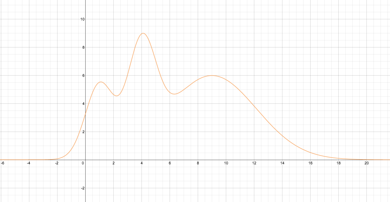
Fig. 25 Initial distribution

Continuous master equations or diffusion equations evolve according to

\[\frac{\partial}{\partial t} P(x,t) = \zeta \frac{\partial}{\partial x} P(x,t) + D \frac{\partial^2}{\partial x^2} P(x,t),\]

given the initial distribution.

In infinite time, the system reach equilibrium.

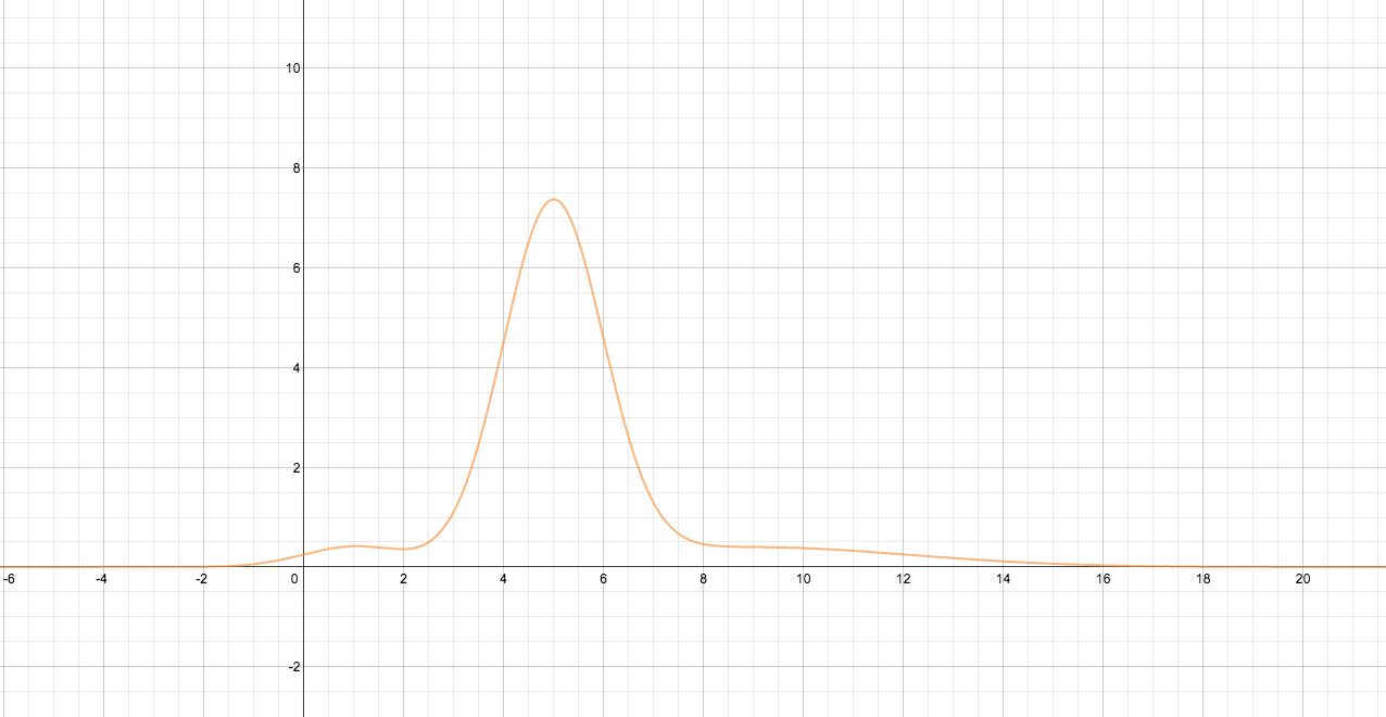
Fig. 26 Final distribution

As long as the system has translational or rotational invariance, we can use Fourier transform to solve the equation.

For \(\zeta =0\), there is only diffusion. Translational invariance is preserved. The Fourier transform for continuous equation is

\[\begin{split}\frac{\partial}{\partial x} e^{ikx}=ike^{ikx} &\implies \frac{\partial}{\partial x} \to ik \\ \frac{\partial^2}{\partial x^2} e^{ikx} = -k^2 e^{ikx} & \implies \frac{\partial^2}{\partial x^2} \to -k^2\end{split}\]

The transformed equation (for \(\zeta=0\) case),

\[\frac{\partial}{\partial t}P^k = -D k^2 P^k\]

and the solution is

\[P^k(t) = P^k(0) e^{-D k^2 t} .\]

To find out the propagator, we complete the square,

\[\begin{split}P(x,t) & = \int P(k,0) e^{-Dk^2t+ikx} dk \\ & = \int P(k,0) e^{-\frac{x^2}{4Dt}} e^{-Dt(k-\frac{ix}{2Dt})^2 }dk \\ & = e^{-\frac{x^2}{4Dt}} \int P(k,0) e^{-Dt(k-\frac{ix}{2Dt})^2 }dk\end{split}\]

The propagator is then

\[\Pi(x,t) = \frac{e^{-\frac{x^2}{4Dt}}}{\sqrt{4\pi Dt}}.\]

Hint

The propagator can also be singular. One of such examples is the logorithm sigularity in 2D.

Bias in Master Equation¶

When \(\zeta\neq 0\), the first term on the right hand side is a decay or viscous term,

\[\frac{\partial}{\partial t}P(x,t) = \zeta \frac{\partial}{\partial x}P(x,t) + D\frac{\partial^2}{\partial x^2}P(x,t).\]

Hint

To check the properties of \(\zeta\), set \(D=0\).

\[\frac{\partial}{\partial t} P = \zeta \frac{\partial}{\partial x} P \Rightarrow P\propto e^{k_w(\omega + \zeta t)}\]

When \(k_w > 0\),

\(\zeta > 0\) : exponential grow;
\(\zeta < 0\) : decay

We can use Fourier transform and complete the square to solve it.

Hint

This formalism is very much like the Gauge Transformation. We define a new derivative

\[\frac{\partial}{\partial x} \to \frac{\partial}{\partial x} + \Gamma(x)\]

Then we plugin this new derivative into diffusion equation,

\[\begin{split}& \frac{\partial}{\partial t} P(x,t) = D\frac{\partial^2}{\partial x^2} P(x,t) \\ \to & \frac{\partial}{\partial t} P(x,t) = D \left(\frac{\partial^2}{\partial x^2} P(x,t) + 2\Gamma\frac{\partial}{\partial x}P(x,t) \right) + D\left( P\left( 2\Gamma^2 + \frac{\partial}{\partial x} \Gamma \right) \right)\end{split}\]

Define \(\zeta := 2\Gamma\), and let \(2\Gamma^2 + \frac{\partial}{\partial x} \Gamma\). [1]_ The diffusion equation under this kind of transformation becomes the one we need.