Information Theory and Statistical Mechanics
Jaynes, E. T. (1957)
Jaynes, E. T. (1957) Information Theory and Statistical Mechanics. Physical Review, 106(4), 620–630. https://doi.org/10.1103/PhysRev.106.620
Line of Reasoning
Jaynes pointed out in this paper that we are solving an insufficient reasoning problem. What we could measure is some macroscopic quantity, from which we derive other macroscopic quantities. That being said, we know a system with a lot of possible microscopic states, \(\{ s_i \}\) while the probabilities of each microscopic state \(\{p_i \}\) is not known at all. We also know a macroscopic quantity \(\langle f(s_i) \rangle\) which is defined as
The question that Jaynes asked was the following.
How are we supposed to find another macroscopic quantity that also depends on the microscopic state of the system? Say \(g(s_i)\).
To visualize this problem, we know think of this landscape of the states. Instead of using the state as the dimensions, we use the probabilities as the dimensions since they are unknown. In the end, we have a coordinate system with each dimension as the value of the probabilities \(\{p_i\}\) and the one dimension for the value of \(\langle g \rangle (p_i)\) which depends on \(\{p_i\}\). Now we constructed a landscape of \(\langle g \rangle (p_i)\). The question is, how does our universe arrange the landscape? Where are we in this landscape if we are at equilibrium?
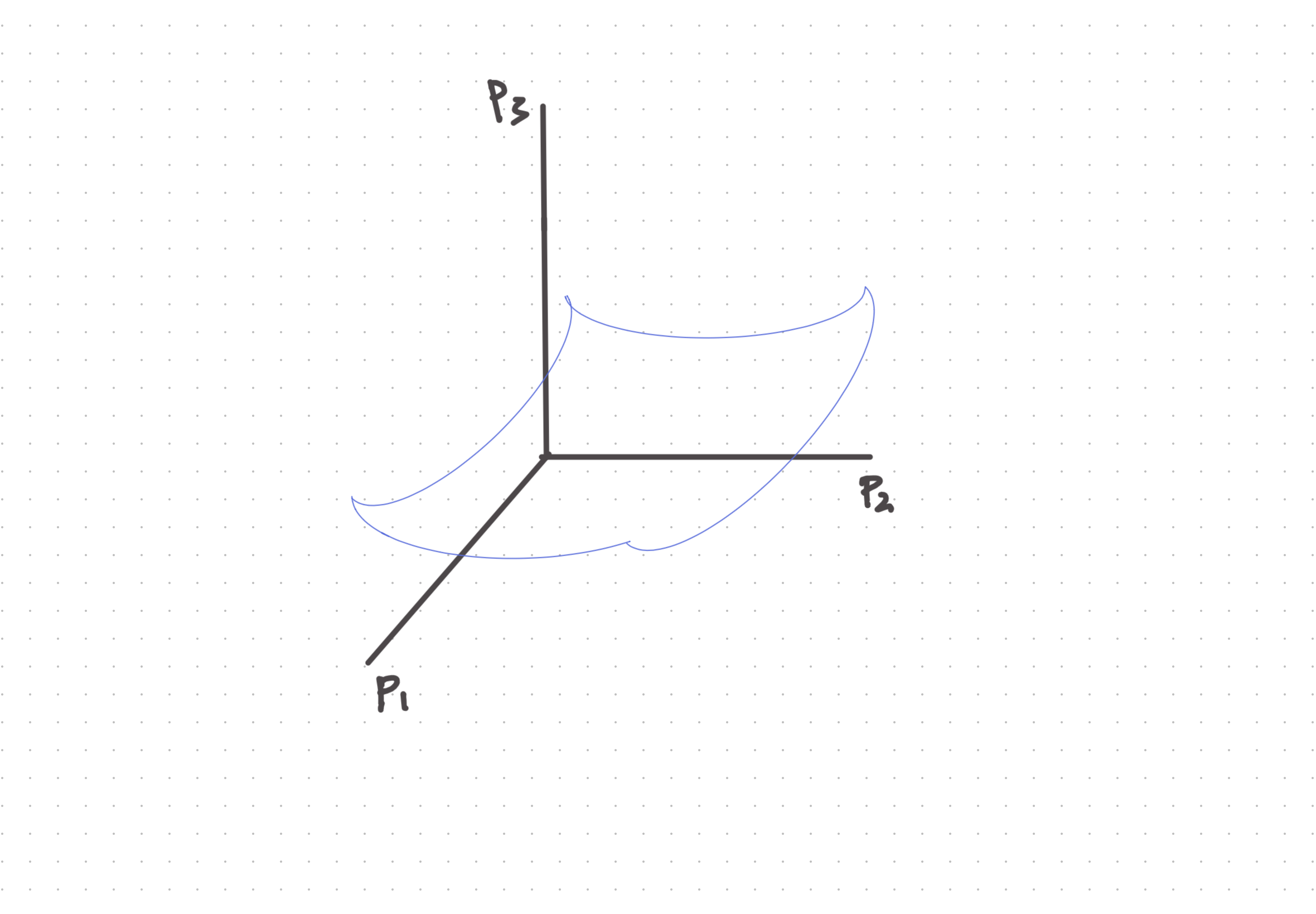
Fig. 39 Illustions.
Crucial Problems
In Jaynes’ paper, he mentioned several crucial problems.
- Do we need to know the landscape formed by \(\{p_i\}\) and \(\langle f(x_i)\rangle\)? No.
- Do we need to find the exact location of our system? We have to.
- How? Using the max entropy principle.
- How to calculate another macroscopic quantity based on one observed macroscopic quantity and the conservation of probability density? Using the probabilities found in the previous step.
- Why does max entropy work from the information point of view? Assuming less about the system.
- Why is the result predicting measurements even the theory is purely objective? This shows how simple nature is. Going philosophical.
- With the generality of the formalism, what else can we do with it to improve our statistical mechanics power? Based on the information we know, we have different formalism of statistical physics.
The Max Entropy Principle
The max entropy principle states that the distribution we choose for our model is based on the least information principle, i.e., largest Shannon entropy \(S_p\), or the distribution \(p(s)\) should have the largest uncertainty, subject to the constraint that the theory should match the observations, i.e., \(\langle f\rangle_{t} = \langle f \rangle_o\) where \(\langle f\rangle_{t}\) denotes for theoretical result and \(\langle f \rangle_o\) is the observation,
We could have multiple constraints,
if we have multiple observables.
Shannon Entropy
The Shannon entropy is
The principle is an optimization problem with constraints. The constraint can be translated into the Lagrange multipliers. The cost function becomes
where the last constraint accounts for the fact that \(p(s)\) has to be a probability density.
Using variational method, we require \(\delta \mathcal L /\delta p = 0\),
The variation of the Shannon entropy is
The variation of the theoretical expectation of the observable is
The variation of the total cost becomes
The solution to this is
By normalizing it, we have the the Boltzmann distribution,
where
This leads to the
Classical Balls on Chessboard
We can write down a function, which is the average of the balls.