Transforms¶

Fourier Transform¶

Fourier transforms are quite useful in solving differential equations. By decomposing the functions using Fourier transform, we might be able to simplify many differential equations.

Suppose we have a differential equation

\[\frac{\partial}{\partial x} f(x) = a g(x).\]

To solve the equation, we decompose \(f(x)\) using its Fourier transform,

\[f(x) = \frac{1}{2\pi} \int_{-\infty}^{\infty} f(k) e^{ikx} dk.\]

Then we get

\[\frac{1}{2\pi}\frac{\partial}{\partial x} \int_{-\infty}^{\infty} f(k) e^{ikx} dk = a \frac{1}{2\pi}\int_{-\infty}^{\infty} g(k) e^{ikx} dk.\]

The equation is then simplified into

\[ik f(k) = a g(k).\]

Note

To summarize, we simple do replacement of the differential operators.

\[\begin{split}\frac{\partial}{\partial x} e^{ikx}=ike^{ikx} &\implies \frac{\partial}{\partial x} \to ik \\ \frac{\partial^2}{\partial x^2} e^{ikx} = -k^2 e^{ikx} & \implies \frac{\partial^2}{\partial x^2} \to -k^2\end{split}\]

Laplace Transform¶

Similar to Fourier transform, Laplace transform is also useful in equation solving.

Laplace transform is a transform of a function of \(t\), e.g. \(f(t)\), to a function of \(s\),

\[\mathscr{L}[f(t)] = \int_0^\infty f(t) e^{ - s t} dt .\]

Some useful properties:

\(\mathscr{L}[\frac{d}{dt}f(t)] = s \mathscr{L}[f(t)] - f(0)\);
\(\mathscr{L}[\frac{d^2}{dt^2}f(t) = s^2 \mathscr{L}[f(t)] - s f(0) - \frac{d f(0)}{dt}\);
\(\mathscr{L}[\int_0^t g(\tau) d\tau ] = \frac{\mathscr{L}[f(t)]}{s}\);
\(\mathscr{L}[\alpha t] = \frac{1}{\alpha} \mathscr{L}[s/\alpha]\);
\(\mathscr{L}[e^{at}f(t)] = \mathscr{L}[f(s-a)]\);
\(\mathscr{L}[tf(t)] = - \frac{d}{ds} \mathscr{L}[f(t)]\).

Some useful results:

\(\mathscr{L}[1] = \frac{1}{s}\);
\(\mathscr{L}[\delta] = 1\);
\(\mathscr{L}[\delta^k] = s^k\);
\(\mathscr{L}[t] = \frac{1}{s^2}\);
\(\mathscr{L}[t^n] = \frac{n!}{s^{n+1}}\)
\(\mathscr{L}[e^{at}]= \frac{1}{s-a}\).

A very nice property of Laplace transform is

\[\begin{split}\mathscr{L}_s [e^{at}f(t)] &= \int_0^\infty e^{-st} e^{-at} f(t) dt \\ & = \int_0^\infty e^{-(s+a)t}f(t) dt \\ & = L_{s+a}[f(t)]\end{split}\]

which is very useful when dealing with master equations.

Two useful results are

\[\mathscr{L}[I_0(2Ft)] = \frac{1}{\sqrt{ \epsilon^2 - (2F)^2 }}\]

and

\[\mathscr{L}[J_0[2Ft]] = \frac{1}{\sqrt{\epsilon^2 + (2F)^2}},\]

where \(I_0(2Ft)\) is the modified Bessel functions of the first kind. \(J_0(2Ft)\) is its companion.

Using the property above, we can find out

\[\mathscr{L}[I_0(2Ft)e^{-2Ft}] = \frac{1}{\sqrt{(\epsilon + 2F)^2 - (2F)^2}} .\]

Example: Solving Differential Equations

For a first order differential equation

\[f'(x) = x,\]

we apply Laplace transform,

\[s F(s) - f(0) = \frac{1}{s^2},\]

from which we solve

\[F(s) = \frac{1}{s^3} + \frac{f(0)}{s}.\]

Then we lookup in the transform table, we find that

\[f(x) = x^2/2 + f(0).\]

Legendre Transform¶

The geometrical meaning of Legendre transformation in thermodynamics can be illustrated by the following graph.

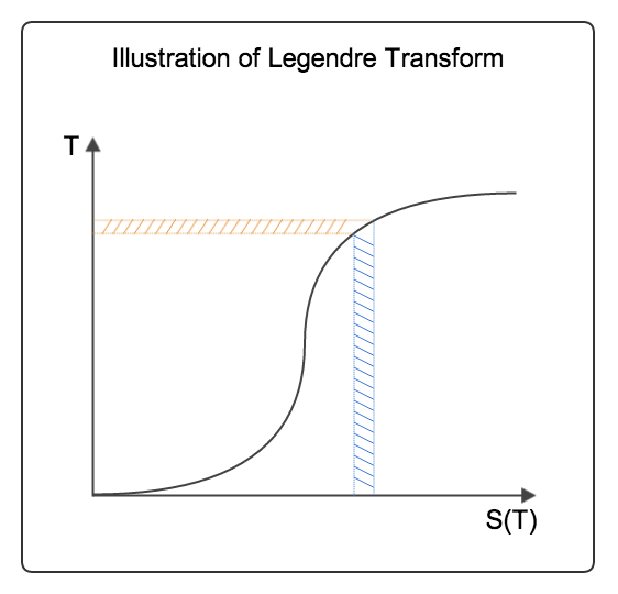
Fig. 4 Legendre transform

In the above example, we know that entropy \(S\) is actually a function of temperature \(T\). For simplicity, we assume that they are monotonically related like in the graph above. When we are talking about the quantity \(T \mathrm d S\) we actually mean the area shaded with blue grid lines. Meanwhile the area shaded with orange line means \(S \mathrm d T\).

Let’s think about the change in internal energy. For this example, we only consider the thermal part,

\[\mathrm d U = T \mathrm d S .\]

Internal energy change is equal to the the area shaded with blue lines. The area shaded with orange lines is the Helmholtz free energy,

\[\mathrm d A = S \mathrm d T .\]

The two quantities \(T \mathrm d S\) and \(S \mathrm d T\) sum up to \(d(TS)\). This is also the area change of the rectangle determined by two edges \(0\) to \(T\) and \(0\) to \(S\).

This is a Legendre transform,

\[\mathrm d U \to \mathrm d A,\]

\[T\mathrm dS \to S \mathrm d T.\]

The point is that \(S(T)\) is a function of \(T\). However, if we know the blue area, we can find out the orange area. This means that the two functions \(A(T)\) and \(U(S)\) are somewhat like a pair. Choosing one of them for a specific calculation is a choice of freedom but we carry all the information in either one once the relation between \(T\) and \(S\) is know.

The above example sheds light on Legendre transform. The mathematical form is a little bit tricky so we will illustrate it using an example. For a function \(U(T, X)\), we find its differential as

\[\mathrm d U(T, X) = \frac{\partial U}{\partial T} \mathrm d T + \frac{\partial U}{\partial X} \mathrm d X.\]

For convinience, we define

\[\begin{split}S =& \frac{\partial U}{\partial T} \\ Y =& \frac{\partial U}{\partial X}.\end{split}\]

The differential of function becomes

\[\mathrm d U(T, X) = S \mathrm dT + Y \mathrm d X,\]

where \(S\) (\(Y\)) and \(T\) (\(X\)) are a conjugate pair.

A Legendre transform says that we change the variable of the differential from \(T\) (\(X\)) to \(S\) (\(Y\)). For example, we know that

\[S \mathrm d T = \mathrm d (ST) - T \mathrm d S.\]

Plugging this into \(\mathrm d U\), we get

\[\mathrm d U(T, X) - \mathrm d(ST) = - T \mathrm dS + Y \mathrm d X.\]

The left hand side is defined as a new differential

\[\mathrm d A(S, X) = \mathrm d ( U(T, X) - ST ).\]

In these calculations, \(U\) is the internal energy and \(A\) is the Helmholtz free energy. The transform that changes the variable from \(X\) to \(Y\) gives us enthalpy \(H\). If we transform both variables then we get Gibbs free energy \(G\). More about these thermodynamic potentials will be discussed in the following chapters.

Refs & Note¶

Zia, Royce K. P., Edward F. Redish and Susan R. McKay. “Making sense of the Legendre transform.” (2009).