Effect of Defects¶

Defects¶

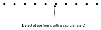
Fig. 29 Defects on a 1D chain

The Smoluchowski Equation describes the distribution of particles in a continuous potential. Here we discuss the distribution of particles in on a chain with defects.

A defect on a chain is a site that captures the walker with a certain probability, as shown in Fig. 29. The master equation that describes the distribution is

(28)¶\[\frac{d}{dt}P_m = F(P_{m+1}+P_{m-1}-2P_m) - C \delta_{m,r} P_m,\]

where \(C\) is the capture rate at the site of defect.

Similar to any other master equations, the (28) is a set of coupled first order differential equations. To solve (28), we consider the following equation

\[\frac{d}{dt}y+\alpha y = f(t).\]

The solution to the above equation when \(\alpha\) is constant, which is

\[y(t) = e^{-\alpha t} y(0) + \int_0^t dt' e^{-\alpha (t - t')} f(t').\]

If we introduce time dependencies for \(\alpha\), we get an extra term \(e^{-\int_{t'}^t ds \alpha(s)}\).

Green’s function

The general solution to any first order differential equation is

\[y(t) = G(t,t_0) y(t_0) + \int_{t_0}^{t} df' G(t,t') f(t').\]

If \(\alpha\) is constant, we use Laplace transform to solve it. Otherwise it is much easier to introduce the Green’s function.

We reformulate the problem to include the initial condition,

\[L[y]\equiv \dot y + \alpha(t)y = f(t), \qquad \text{for } a < t, \qquad y(a) = 0.\]

The solution is

\[y = \int_a^\infty G(t\vert \xi)f (\xi) d\xi,\]

where the Green’s function \(G(t\vert \xi)\) is defined by

\[L[G(t\vert \xi)] = \delta(t - \xi), \qquad \text{for } a < t, \qquad G(a\vert \xi) = 0.\]

In this specific case, Green function is

\[G(x\vert \xi) = e^{-\int_\xi^x \alpha(t) dt} H(t - \xi),\]

where \(H\) is the Heaviside function.

For first order differential equations, it is much easier to use the general solution

\[y(t) = \frac{\int\mu(t) f(t) dt + C}{\mu(t)},\]

where \(\mu(t) := e^{\int \alpha(t') dt'}\).

However, when dealing with more complicate differential equations, the Green’s function method becomes more useful and intuitive. Green’s function represents the impulse response of the dynamical system.

More about Green’s function, for example, the solution to second order inhomogeneous equation, is found in Green’s Function.

A more general problem is a time dependent source \(g_m(t)\) in the master equation,

\[\frac{d}{dt}P_m = F(P_{m+1} + P_{m-1} - 2P_m) + g_m(t).\]

The formal solution is

\[P_m(t) = \eta_m(t) + \int_0^t dt'\sum_n \Pi_{m-n}(t-t') g(t').\]

However, the solution is still coupled to other sites. We apply Fourier transform on it to detangle the spatial coupling,

\[P^k(t) = \eta^k(t) + \int_0^t dt' \Pi^k(t-t') g^k(t').\]

To simplify the result, Laplace transform is used,

\[\tilde P^k = \tilde \eta^k + \tilde \Pi^k \tilde g^k .\]

Laplace Transform

Laplace transform is a transform of a function \(f(t)\) to a function of \(s\) through

\[L[f(t)] = \int_0^\infty f(t) e^{ - s t} dt .\]

Some useful properties of Laplace transform are listed below.

\(L[\frac{d}{dt}f(t)] = s L[f(t)] - f(0)\);
\(L[\frac{d^2}{dt^2}f(t) = s^2 L[f(t)] - s f(0) - \frac{d f(0)}{dt}\);
\(L[\int_0^t g(\tau) d\tau ] = \frac{L[f(t)]}{s}\);
\(L[\alpha t] = \frac{1}{\alpha} L[s/\alpha]\);
\(L[e^{at}f(t)] = L[f(s-a)]\);
\(L[tf(t)] = - \frac{d}{ds} L[f(t)]\).

Some useful results of Laplace transform on some simple functions are calculated.

\(L[1] = \frac{1}{s}\);
\(L[\delta] = 1\);
\(L[\delta^k] = s^k\);
\(L[t] = \frac{1}{s^2}\);
\(L[e^{at}]= \frac{1}[s-a]\).

More on Laplace transform is in Laplace Transform.

Transform back into real space,

(29)¶\[\tilde P_m(\epsilon) = \tilde \eta_m(\epsilon) + \sum_n \tilde \Pi_{m-n}(\epsilon) \tilde g_n(\epsilon).\]

To get the solution to (28), we simply define

\[\tilde g_n = - C\delta _{n,r} \tilde P_n\]

and plugin it back into (29), we get

(30)¶\[\tilde P_m = \tilde \eta _m - C \tilde \Pi_{m-r} \tilde P_r .\]

In fact, we haven’t solved the equation. The solution (30) is merely a formal solution. The right hand side still depends on the probabillity.

If we set \(m=r\), we get remove the dependencis of the mth mode,

\[\tilde P_r = \tilde \eta_r - C\tilde \Pi_0 \tilde P_r .\]

From which, we fine the solution to the rth component is,

\[\tilde P_r = \frac{\tilde \eta_r}{1+C\tilde \Pi_0} .\]

The rth mode is then combined with (30),

\[\begin{split}\tilde P_m &= \eta_m - C\tilde \Pi_{m-r} \frac{\tilde \eta_r}{1+C\tilde \Pi_0} \\ & = \eta_m - \frac{\tilde \Pi_{m-r} \eta_r}{1/C + \tilde \Pi_0}\end{split}\]

Take the limits to check the properties.

Motion limit is given by

\[\frac{1}{C} \ll \tilde \Pi_0 .\]

In this case, \(\tilde P_m \to \tilde \eta_m - \frac{\tilde \Pi_{m-r} \tilde \eta_r}{\tilde \Pi_0}\). In this limit, the propagator decreases with time so fast that it becomes small enough to be neglected. The survival probability is dominated by motion not the capture.
Capture limit is given by

\[\frac{1}{C} \gg \tilde \Pi_0 .\]

In this limit, the survival probability is dominated by capture, \(\tilde P_m \to \tilde \eta_m\).

Numerical Solution

Numerical solution to this is straight forward.

A Brief Summary of the Effect of Defect

The master equation is

\[\frac{d}{dt} P_m = \text{Without Defect} - C \delta_{m,r} P_m.\]

The propagator, aka the Green’s function, is \(\Pi_{m-n}(t,t_0)\). Apply Laplace transform,

\[\tilde P_m(\epsilon) = \tilde \eta_m(\epsilon) - C\tilde \Pi_{m-r}(\epsilon) \tilde P_r(\epsilon).\]

Substitute of \(m\) with \(r\), we get

\[\tilde P_r(\epsilon) = \frac{\tilde \eta_m(\epsilon)}{1+ \tilde \Pi_0(\epsilon)}.\]

This result is then plugged back to the solution, the final solution becomes

\[\tilde P_m(\epsilon) = \tilde \eta_m(\epsilon) - C\tilde \Pi_{m-r}(\epsilon) \tilde \eta_r(t) \frac{1}{1+C\tilde \Pi(\epsilon)}.\]

The survival probability is defined as

\[Q(t) = \sum_m P_m .\]

Then we can find out its Laplace transform, which is

\[\tilde Q(t) = \frac{1}{\epsilon} \left[ 1 - \frac{\tilde \eta_r(\epsilon)}{1/C + \tilde \Pi_0} \right]\]

Survival Probability¶

The survival probability of a particle is the summation of the probabilities at all the sites,

\[Q(t) = \sum_n P_m(t),\]

i.e.,

\[\tilde Q(t) = \sum_m \tilde P_m = \frac{1}{\epsilon}\left( 1 - \frac{\tilde \eta_r}{1/C + \tilde \Pi_0} \right)\]

Looking through the table of Laplace transform,

\[\frac{d}{dt}Q \to \tilde Q - 1.\]

The survival probability is then calculated as

\[\frac{d}{dt}Q(t) = - \int_0^t dt' \mathscr M(t-t') \eta(t')\]

in which

\[\mathscr M(t-t') = \frac{1}{1/C + \tilde \Pi_0} .\]

Hint

The Laplace transform of propagator is

\[\tilde \Pi_0 = \int_0^\infty e^{-\epsilon t} \Pi_0 dt,\]

which is actually decreasing when \(\Pi_0\) is a constant.

Photosynthesis¶

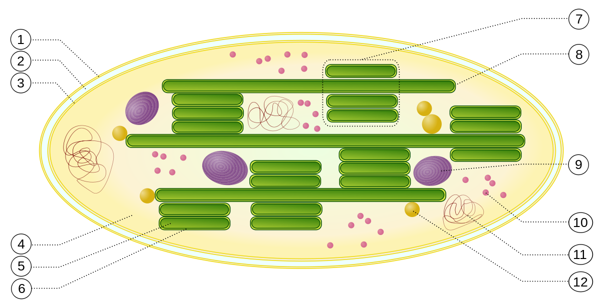
Fig. 30 Captions are here on wikipedia. Chloroplast ultrastructure: 1. outer membrane 2. intermembrane space 3. inner membrane (1+2+3: envelope) 4. stroma (aqueous fluid) 5. thylakoid lumen (inside of thylakoid) 6. thylakoid membrane 7. granum (stack of thylakoids) 8. thylakoid (lamella) 9. starch 10. ribosome 11. plastidial DNA 12. plastoglobule (drop of lipids)

The obsorbed energy of photons follows a random walk in the chloroplast until it hits on a reaction center. On the other hand, the photons can also be emited after some time. The whole process is a master equation of the form

\[\frac{d}{dt} P_m = \text{Without reaction and emission} - C\delta_{m,r} P_m - \frac{P_m}{\tau},\]

where the last term \(\frac{P_m}{\tau}\) is describes the emission.

What the experimentalists are interested in is a quantity called quantum yield, which is defined as

\[\begin{split}\text{quantum yield} & = \frac{\text{ Number of excitations in the trap or reaction center } }{\text{Number of total excitations}}\\ & = \frac{\text{Integration of survival probability with the reaction center}}{\text{Integration of survival probability without the raction center}} .\end{split}\]

Without the reaction,

(31)¶\[\frac{d}{dt}Q + \frac{Q}{\tau} = 0,\]

Assume the survival probability to have the following form

\[Q(t) = Q(0) e^{-t/\tau}.\]

(31) becomes,

\[\frac{1}{\tau} \int_0^\infty Q(t) dt = 1 .\]

The quantum yield is

\[\text{quantum yield} = \frac{\frac{1}{\tau} \int_0^\infty dt Q(t) \vert_{\text{with traps}} }{\frac{1}{\tau} \int_0^\infty dt Q(t) \vert_{\text{without traps}} } .\]

The integrals are complex. Forturnatedly, the inverse Laplace transform is not needed since

\[\int_0^\infty Q(t) dt = L_{\epsilon=0}[Q(t)] .\]

Define the quantities without traps to be the prime quantities. We define a new quantity

\[\bar P_m = e^{t/\tau} P_m'.\]

\(\bar P_m\) reduces the master equation to the case without emissions which has already been solved,

\[\bar P_m = P_m.\]

Finally, the survival probability with traps is

\[Q' = e^{-t/\tau} Q.\]

Integrate over time \(t\),

\[\begin{split}\int_0^\infty Q'(t) dt &= \int_0^\infty e^{-t/\tau} Q(t) dt \\ & = L_{\epsilon=1/\tau} [Q(t)].\end{split}\]

This result simplifies our calculation because the survival probability in the case of traps is not needed with Laplace transform of \(Q(t)\),

\[\tilde Q(\epsilon) = \frac{1}{\epsilon} \left( 1- \frac{\tilde \eta}{1/C + 1/\sqrt{\epsilon(\epsilon +4F)}} \right).\]

We have

\[\begin{split}\frac{1}{\tau}\int_0^\infty dt Q(t) &= L_{\epsilon=0}[Q(t)] = \tilde Q(\epsilon=0) \\ \frac{1}{\tau}\int_0^\infty dt Q'(t) &= L_{\epsilon=1/\tau}[Q'(t)] = \tilde Q(\epsilon=\frac{1}{\tau}).\end{split}\]

The initial condition is used in \(\tilde \eta (\epsilon) = \tilde \Pi_{m-r}(\epsilon) P_m(0)\).

Multiple Defects¶

The problem is generalized into include multiple defects. For example, the two defects case is described by

\[\frac{d}{dt}P_m = \cdots - C_r\delta_{m,r}P_m - C_s \delta_{m,s} P_m.\]

Similar to the single defect case, we solve the two special modes by setting \(m=r\) and \(m=s\). Two equations of \(\tilde P_r\) and \(\tilde P_s\) are observed,

\[\begin{split}\tilde P_r &= \eta_r - C_r \tilde \Pi_0 \tilde P_r - C_s \tilde \Pi_{r-s} \tilde P_r \\ \tilde P_s = \eta_s - C_r \tilde \Pi_{s-r} \tilde P_s - C_s \tilde \Pi_0 \tilde P_s.\end{split}\]

To a physicist, the problem gets quite complicated as the number of defects becomes larger.