Ensembles¶

In statistical mechanics, only partial information of the system can be observed. From a macroscopic point of view, thermodynamic observables do not tell us about all the information of the microstates. The contimiuum in the phase space, aka, the phase space distributions, is used to represent the internal stuctures of the system. For equlibrium physics, the probability distribution of the microstates \(\rho(\{p_i\}, \{q_i\})\) may be used to calculate the macroscopic observables \(\mathscr O\), i.e., \(\langle \mathscr O \rangle (t) = \int \mathscr O (\{p_i\}, \{q_i\}) \rho(\{p_i\}, \{q_i\}) d\Omega\). The question is how to obtain the probability density \(\rho(\{p_i\}, \{q_i\})\), i.e., the probability density distribution of phases space points. In the language of statistics, we either invent a know-all theory which involves the whole population of microscopic states, or a good sampling method to sample some representative microstates.

In Boltzmann’s theory, this problem is solved by applying the least information assumption, i.e., equal a priori principle. Using this, Boltzmann found better ways of calculating the observable by deriving the probabilities of the single particle energy states. A distribution in Boltzmann’s theory is shown in the following table.

single particle energy	number of microstates	degeneracy
\(e_1\)	\(n_1\)	\(g_1\)
\(e_2\)	\(n_2\)	\(g_2\)
\(e_3\)	\(n_3\)	\(g_3\)
…	…	…
\(e_i\)	\(n_i\)	\(g_i\)
…	…	…

The most probable distribution, i.e., the distribution that appears the most frequently, shall be used to calculate the thermodynamic observables. With this, it has been assumed that the system is dynamically moving in the phase space but is close to most probable distribution most of the time. This is our sampling method and the most probable distribution is our statistical sample. It sounds too extreme to use one distribution as a statistical sample. However, the macroscopic observables barely fluctuates because the most probable distribution is a delta-like distribution.

However, single particle energy states are not clearly defined in systems with strong self-interactions. In such systems, probabilities of microstates on the different distributions of single particle energy states shall not be defined either.

This problem is solved by the ensemble methods. Instead of collecting statistical sampling on the different microstates in time dimension, we make virtual copies of the system, aka replicas, so that we sample among these virtual copies. The replicas are interacting with each other as well as the environment of the original lab system. The energies of the replicas are denoted as \(E_i\). The number of replicas on each energy \(E_i\) is denoted as \(n_i\). There will be multiple ways of configuring the ensemble so that it satisfies our thermodynamic conditions. A distribution in ensemble theory is shown in the following table.

replica energy	number of replcas	degeneracy
\(E_1\)	\(N_1\)	\(G_1\)
\(E_2\)	\(N_2\)	\(G_2\)
\(E_3\)	\(N_3\)	\(G_3\)
…	…	…
\(E_i\)	\(N_i\)	\(G_i\)
…	…	…

The most probable distribution shall be used as a statistical sample to calculate the thermodynamic observables.

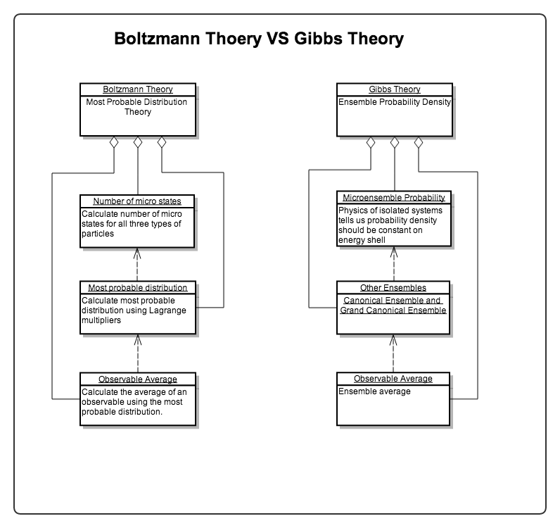
A compare Boltzmann theory and ensemble theory is shown in the following chart.

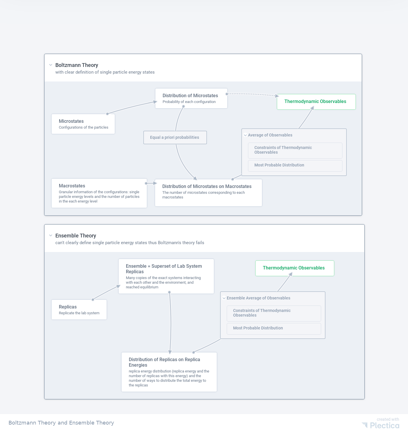
../_images/boltzmann-theory-and-ensemble-theory.png

Fig. 19 Comparing Boltzmann theory and ensemble theory. Download the PDF version: Boltzmann theory and ensemble theory.

Code of the Chart

Here is the JSON being used to generate the charts on Plectica.com.

{"id":380580,"title":"Boltzmann Theory and Ensemble Theory","version_number":0,"owner_user_id":15074,"operation_sequence":11473162,"workspace":null,"is_public":1,"roles":{"card":{"role":"card","displayName":"Card","attributes":[]}},"map_data":{"nodes":[{"id":"5429660568700902","title":"Microstates","summary":"Configurations of the particles","titleMeta":[],"summaryMeta":[],"description":null,"x":24,"y":112.50362792968772,"height":69,"isCollapsed":false,"parentId":"8590816235785074","createdById":15074,"orderIndex":1,"canonicalNodeUUID":"2216537070500096","externalIdentifier":null,"librarySlug":null,"layoutName":"layout-row","linkStates":{},"parentId0":"8590816235785074","canonicalNodeId":"2216537070500096"},{"id":"38555982454854","title":"Macrostates","summary":"Granular information of the configurations: single particle energy levels and the number of particles in the each energy level","titleMeta":[],"summaryMeta":[],"description":null,"x":24,"y":334.2251794433596,"height":69,"isCollapsed":false,"parentId":"8590816235785074","createdById":15074,"orderIndex":5,"canonicalNodeUUID":"3215286425700970","externalIdentifier":null,"librarySlug":null,"layoutName":"layout-row","linkStates":{},"parentId0":"8590816235785074","canonicalNodeId":"3215286425700970"},{"id":"5893191289108180","title":"Thermodynamic Observables","summary":"","titleMeta":[],"summaryMeta":null,"description":null,"x":798.1256408691404,"y":44.40115251813635,"height":53,"isCollapsed":false,"parentId":"8590816235785074","createdById":15074,"orderIndex":3,"canonicalNodeUUID":"4647486971351130","externalIdentifier":null,"librarySlug":null,"layoutName":"layout-row","backgroundColor":"#09a65f","displayStyle":"standard","linkStates":{},"parentId0":"8590816235785074","canonicalNodeId":"4647486971351130"},{"id":"91175769756342","title":"Distribution of Microstates","summary":"Probability of each configuration","titleMeta":[],"summaryMeta":[],"description":null,"x":380.41644478934114,"y":24,"height":69,"isCollapsed":false,"parentId":"8590816235785074","createdById":15074,"orderIndex":0,"canonicalNodeUUID":"2209983646496592","externalIdentifier":null,"librarySlug":null,"layoutName":"layout-row","linkStates":{},"parentId0":"8590816235785074","canonicalNodeId":"2209983646496592"},{"id":"3752942348728678","title":"Distribution of Microstates on Macrostates","summary":"The number of microstates corresponding to each macrostates","titleMeta":[],"summaryMeta":[],"description":null,"x":379.3568507603236,"y":336.74313743954656,"height":85,"isCollapsed":false,"parentId":"8590816235785074","createdById":15074,"orderIndex":4,"canonicalNodeUUID":"3936591638560858","externalIdentifier":null,"librarySlug":null,"layoutName":"layout-row","userHeight":93.90388997395837,"userWidth":367.32682291666663,"linkStates":{},"parentId0":"8590816235785074","canonicalNodeId":"3936591638560858"},{"id":"8590816235785074","title":"Boltzmann Theory","summary":"with clear definition of single particle energy states","titleMeta":[],"summaryMeta":[],"description":null,"x":270.82055646623917,"y":59.473311244419385,"height":554.78125,"isCollapsed":false,"parentId":null,"createdById":15074,"orderIndex":0,"canonicalNodeUUID":"1061380107998244","externalIdentifier":null,"librarySlug":null,"layoutName":"layout-freehand","linkStates":{},"canonicalNodeId":"1061380107998244"},{"id":"3643453456996428","title":"Replicas","summary":"Replicate the lab system ","titleMeta":[],"summaryMeta":[],"description":null,"x":24,"y":164.28682256105543,"height":69,"isCollapsed":false,"parentId":"8678627374434140","createdById":15074,"orderIndex":0,"canonicalNodeUUID":"3213113326411440","externalIdentifier":null,"librarySlug":null,"layoutName":"layout-row","linkStates":{},"parentId0":"8678627374434140","canonicalNodeId":"3213113326411440"},{"id":"893268972350116","title":"Ensemble = Superset of Lab System Replicas","summary":"Many copies of the exact systems interacting with each other and the environment, and reached equilibrium","titleMeta":[],"summaryMeta":[],"description":null,"x":254.06968925617116,"y":24,"height":121,"isCollapsed":false,"parentId":"8678627374434140","createdById":15074,"orderIndex":1,"canonicalNodeUUID":"1318555306680688","externalIdentifier":null,"librarySlug":null,"layoutName":"layout-row","linkStates":{},"parentId0":"8678627374434140","canonicalNodeId":"1318555306680688"},{"id":"4804819707770512","title":"Thermodynamic Observables","summary":"","titleMeta":null,"summaryMeta":null,"description":null,"x":724.4424691767326,"y":30.163697478991786,"height":52,"isCollapsed":false,"parentId":"8678627374434140","createdById":15074,"orderIndex":4,"canonicalNodeUUID":"1348366312564316","externalIdentifier":null,"librarySlug":null,"layoutName":"layout-row","backgroundColor":"#09a65f","displayStyle":"standard","linkStates":{},"parentId0":"8678627374434140","canonicalNodeId":"1348366312564316"},{"id":"6751053013997652","title":"Distribution of Replicas on Replica Energies","summary":"replica energy distribution (replica energy and the number of replicas with this energy) and the number of ways to distribute the total energy to the replicas","titleMeta":[],"summaryMeta":[],"description":null,"x":264.57319415813237,"y":345.87021510361984,"height":85,"isCollapsed":false,"parentId":"8678627374434140","createdById":15074,"orderIndex":3,"canonicalNodeUUID":"3483689088913384","externalIdentifier":null,"librarySlug":null,"layoutName":"layout-row","linkStates":{},"parentId0":"8678627374434140","canonicalNodeId":"3483689088913384"},{"id":"8236492870889286","title":"Equal a priori probabilities","summary":"","titleMeta":[],"summaryMeta":null,"description":null,"x":710.9536303277997,"y":336.7655813450129,"height":42.71875,"isCollapsed":false,"parentId":null,"createdById":15074,"orderIndex":0,"canonicalNodeUUID":"6426202418936556","externalIdentifier":null,"librarySlug":null,"layoutName":"layout-row","linkStates":{},"canonicalNodeId":"6426202418936556"},{"id":"1374922614344530","title":"Average of Observables","summary":"","titleMeta":[],"summaryMeta":[],"description":null,"x":1121.4605366988371,"y":334.85714841247864,"height":160.0625,"isCollapsed":false,"parentId":null,"createdById":15074,"orderIndex":0,"canonicalNodeUUID":"402044386490722","externalIdentifier":null,"librarySlug":null,"layoutName":"layout-row","linkStates":{},"canonicalNodeId":"402044386490722"},{"id":"7160646853346752","title":"Constraints of Thermodynamic Observables","summary":"","titleMeta":[],"summaryMeta":null,"description":null,"x":0,"y":0,"height":61,"isCollapsed":false,"parentId":"1374922614344530","createdById":15074,"orderIndex":1,"canonicalNodeUUID":"3263781844877632","externalIdentifier":null,"librarySlug":null,"layoutName":"layout-row","linkStates":{},"parentId0":"1374922614344530","canonicalNodeId":"3263781844877632"},{"id":"8957829856375302","title":"Most Probable Distribution","summary":"","titleMeta":[],"summaryMeta":null,"description":null,"x":0,"y":0,"height":45,"isCollapsed":false,"parentId":"1374922614344530","createdById":15074,"orderIndex":2,"canonicalNodeUUID":"4531556412633654","externalIdentifier":null,"librarySlug":null,"layoutName":"layout-row","linkStates":{},"parentId0":"1374922614344530","canonicalNodeId":"4531556412633654"},{"id":"8678627374434140","title":"Ensemble Theory","summary":"can't clearly define single particle energy states thus Boltzmann's theory fails","titleMeta":[],"summaryMeta":[],"description":null,"x":270.11747455466576,"y":645.6615329432553,"height":558.421875,"isCollapsed":false,"parentId":null,"createdById":15074,"orderIndex":0,"canonicalNodeUUID":"3286139737046258","externalIdentifier":null,"librarySlug":null,"layoutName":"layout-freehand","cx":0,"cy":0,"uh":460.3409179687501,"uw":1097.299853515625,"linkStates":{},"canonicalNodeId":"3286139737046258"},{"id":"6904809577401286","title":"Ensemble Average of Observables","summary":"","titleMeta":[],"summaryMeta":[],"description":null,"x":1053.0230718813957,"y":893.505635348629,"height":160.0625,"isCollapsed":false,"parentId":null,"createdById":15074,"orderIndex":0,"canonicalNodeUUID":"6450557267461878","externalIdentifier":null,"librarySlug":null,"layoutName":"layout-row","linkStates":{},"canonicalNodeId":"6450557267461878"},{"id":"4439272904131590","title":"Constraints of Thermodynamic Observables","summary":"","titleMeta":[],"summaryMeta":null,"description":null,"x":0,"y":0,"height":61,"isCollapsed":false,"parentId":"6904809577401286","createdById":15074,"orderIndex":1,"canonicalNodeUUID":"3997271437510356","externalIdentifier":null,"librarySlug":null,"layoutName":"layout-row","linkStates":{},"parentId0":"6904809577401286","canonicalNodeId":"3997271437510356"},{"id":"56641628703632","title":"Most Probable Distribution","summary":"","titleMeta":[],"summaryMeta":null,"description":null,"x":0,"y":0,"height":45,"isCollapsed":false,"parentId":"6904809577401286","createdById":15074,"orderIndex":2,"canonicalNodeUUID":"8327434325216788","externalIdentifier":null,"librarySlug":null,"layoutName":"layout-row","linkStates":{},"parentId0":"6904809577401286","canonicalNodeId":"8327434325216788"}],"links":[{"id":"1677151318953608","fromNodeId":"3643453456996428","toNodeId":"893268972350116","linkNodeId":null,"createdById":15074,"angleStartToR":-0.06544984694978735,"angleEndToR":0.06544984694978735,"direction":"right","lineCurvature":"arc"},{"id":"2147817250009962","fromNodeId":"38555982454854","toNodeId":"3752942348728678","linkNodeId":null,"createdById":15074,"angleStartToR":-0.06544984694978735,"angleEndToR":0.06544984694978735,"direction":"right","lineCurvature":"arc"},{"id":"246476602621234","fromNodeId":"893268972350116","toNodeId":"6751053013997652","linkNodeId":null,"createdById":15074,"angleStartToR":-0.06544984694978735,"angleEndToR":0.06544984694978735,"direction":"right","lineCurvature":"arc"},{"id":"2806905245085312","fromNodeId":"3752942348728678","toNodeId":"5893191289108180","linkNodeId":"1374922614344530","createdById":15074,"angleStartToR":0.11424656578134328,"angleEndToR":-0.3038950011833439,"direction":"right","lineCurvature":"arc"},{"id":"3629939143258684","fromNodeId":"6751053013997652","toNodeId":"4804819707770512","linkNodeId":"6904809577401286","createdById":15074,"angleStartToR":0.08322371282495183,"angleEndToR":-0.2862632564870031,"direction":"right","lineCurvature":"arc"},{"id":"3992308683561910","fromNodeId":"91175769756342","toNodeId":"5893191289108180","linkNodeId":"361523799837588","createdById":15074,"angleStartToR":-0.06987676226149359,"angleEndToR":0.0930958387590537,"direction":"right","lineType":"dotted","lineCurvature":"arc"},{"id":"5178144180868412","fromNodeId":"5429660568700902","toNodeId":"91175769756342","linkNodeId":null,"createdById":15074,"angleStartToR":-0.06544984694978735,"angleEndToR":0.06544984694978735,"direction":"right","lineCurvature":"arc"},{"id":"6341373670204238","fromNodeId":"91175769756342","toNodeId":"3752942348728678","linkNodeId":"8236492870889286","createdById":15074,"angleStartToR":0.566118903191613,"angleEndToR":-0.3926886055023908,"direction":"right","lineCurvature":"arc"}],"deleted":{"nodes":[{"id":"3500200833686730","title":"","summary":"","titleMeta":[],"summaryMeta":null,"description":null,"x":0,"y":0,"height":59,"isCollapsed":false,"parentId":"5429660568700902","createdById":15074,"orderIndex":1,"canonicalNodeUUID":"6551004396395208","externalIdentifier":null,"librarySlug":null,"layoutName":"layout-row","linkStates":{}},{"id":"4506670361559150","title":"","summary":"","titleMeta":null,"summaryMeta":null,"description":null,"x":0,"y":0,"height":59,"isCollapsed":false,"parentId":"5429660568700902","createdById":15074,"orderIndex":2,"canonicalNodeUUID":"482404133000310","externalIdentifier":null,"librarySlug":null,"layoutName":"layout-row","linkStates":{}},{"id":"4060418982148924","title":"Probabilities","summary":"probabilities of the macrostates","titleMeta":[],"summaryMeta":[],"description":null,"x":740.2147442362602,"y":456.14135929081795,"height":60,"isCollapsed":false,"parentId":null,"createdById":15074,"orderIndex":0,"canonicalNodeUUID":"8990463552879476","externalIdentifier":null,"librarySlug":null,"layoutName":"layout-row","linkStates":{}},{"id":"6777445516919772","title":"Probabilities","summary":"Probabilities of microstates","titleMeta":[],"summaryMeta":[],"description":null,"x":793.951882997135,"y":294.6305837198761,"height":116.6875,"isCollapsed":false,"parentId":null,"createdById":15074,"orderIndex":0,"canonicalNodeUUID":"7286219457633132","externalIdentifier":null,"librarySlug":null,"layoutName":"layout-row","linkStates":{}},{"id":"1518195147793154","title":"","summary":"","titleMeta":null,"summaryMeta":null,"description":null,"x":0,"y":0,"height":45,"isCollapsed":false,"parentId":"4060418982148924","createdById":15074,"orderIndex":1,"canonicalNodeUUID":"7837909491675786","externalIdentifier":null,"librarySlug":null,"layoutName":"layout-row","linkStates":{}},{"id":"7090555377563712","title":"","summary":"","titleMeta":null,"summaryMeta":null,"description":null,"x":0,"y":0,"height":45,"isCollapsed":false,"parentId":"4060418982148924","createdById":15074,"orderIndex":2,"canonicalNodeUUID":"3358987022024774","externalIdentifier":null,"librarySlug":null,"layoutName":"layout-row","linkStates":{}},{"id":"6450263253144610","title":"Calculation is Hard","summary":"","titleMeta":[],"summaryMeta":[],"description":null,"x":0,"y":0,"height":45,"isCollapsed":false,"parentId":"6777445516919772","createdById":15074,"orderIndex":-0.5,"canonicalNodeUUID":"6028341441338950","externalIdentifier":null,"librarySlug":null,"layoutName":"layout-row","linkStates":{}},{"id":"1895165448100790","title":"Boltzmann Distribution","summary":"","titleMeta":[],"summaryMeta":null,"description":null,"x":0,"y":0,"height":45,"isCollapsed":false,"parentId":"4060418982148924","createdById":15074,"orderIndex":1,"canonicalNodeUUID":"4918054235209930","externalIdentifier":null,"librarySlug":null,"layoutName":"layout-row","linkStates":{}},{"id":"3755075907434656","title":"","summary":"","titleMeta":[],"summaryMeta":null,"description":null,"x":202.11656511579216,"y":200.851093226842,"height":87,"isCollapsed":false,"parentId":"8590816235785074","createdById":15074,"orderIndex":2,"canonicalNodeUUID":"5883238193815276","externalIdentifier":null,"librarySlug":null,"layoutName":"layout-row","linkStates":{}},{"id":"8045637202702396","title":"","summary":"","titleMeta":null,"summaryMeta":null,"description":null,"x":124.820068359375,"y":24,"height":53,"isCollapsed":false,"parentId":"8590816235785074","createdById":15074,"orderIndex":6,"canonicalNodeUUID":"7398883742675414","externalIdentifier":null,"librarySlug":null,"layoutName":"layout-row","linkStates":{}},{"id":"361523799837588","title":"","summary":"","titleMeta":null,"summaryMeta":null,"description":null,"x":1026.4852806953932,"y":282.8184787475733,"height":0,"isCollapsed":false,"parentId":null,"createdById":15074,"orderIndex":0,"canonicalNodeUUID":"7893742733961018","externalIdentifier":null,"librarySlug":null,"layoutName":"layout-row","linkStates":{}},{"id":"8868736432189276","title":"","summary":"","titleMeta":[],"summaryMeta":null,"description":null,"x":299.75974596244737,"y":347.2722689075624,"height":71,"isCollapsed":false,"parentId":"8678627374434140","createdById":15074,"orderIndex":2,"canonicalNodeUUID":"6606211448969334","externalIdentifier":null,"librarySlug":null,"layoutName":"layout-row","linkStates":{}}],"links":[{"id":"1059210666622488","fromNodeId":"38555982454854","toNodeId":"5893191289108180","linkNodeId":"4060418982148924","createdById":15074,"angleStartToR":-0.09252957341193704,"angleEndToR":-6.212015592978304,"direction":"right","lineCurvature":"arc"},{"id":"241561742597516","fromNodeId":"8868736432189276","toNodeId":"6751053013997652","linkNodeId":null,"createdById":15074,"angleStartToR":-0.06544984694978735,"angleEndToR":0.06544984694978735,"direction":"right","lineCurvature":"arc"},{"id":"2573943194018260","fromNodeId":"3755075907434656","toNodeId":"3752942348728678","linkNodeId":null,"createdById":15074,"angleStartToR":-0.06544984694978735,"angleEndToR":0.06544984694978735,"direction":"right","lineCurvature":"arc"},{"id":"2593314818010554","fromNodeId":"3755075907434656","toNodeId":"5893191289108180","linkNodeId":null,"createdById":15074,"angleStartToR":0,"angleEndToR":null,"direction":"right","lineCurvature":"arc"},{"id":"2614172271234618","fromNodeId":"38555982454854","toNodeId":"3755075907434656","linkNodeId":null,"createdById":15074,"angleStartToR":-0.06544984694978735,"angleEndToR":0.06544984694978735,"direction":"right","lineCurvature":"arc"},{"id":"3810274950159542","fromNodeId":"5429660568700902","toNodeId":"5893191289108180","linkNodeId":"6777445516919772","createdById":15074,"angleStartToR":-0.07721488249279425,"angleEndToR":0.08042798457933564,"direction":"right","lineCurvature":"arc"},{"id":"4231797360040166","fromNodeId":"5429660568700902","toNodeId":"3755075907434656","linkNodeId":null,"createdById":15074,"angleStartToR":-0.06544984694978735,"angleEndToR":0.06544984694978735,"direction":"right","lineCurvature":"arc"},{"id":"4537266285073968","fromNodeId":"893268972350116","toNodeId":"4804819707770512","linkNodeId":null,"createdById":15074,"angleStartToR":0,"angleEndToR":null,"direction":"right","lineCurvature":"arc"}],"perspectives":[],"presentations":[]},"display_properties":null,"perspectives":[],"presentations":[],"regions":[],"urlPreviews":[],"comments":[]},"owner_user":{"id":15074,"display_name":"Lei Ma","avatar_url":"https://lh3.googleusercontent.com/a-/AAuE7mC-NmNVBKYMyoHb2W5jdLcdrNyWZ-LspLwSn7qBgA","created_time":"2019-03-21T21:57:54.000Z","member_since":"March 21st 2019"},"collaborators":[{"id":11464472,"user_id":15074,"activity_count":249,"created_time":"2019-12-27T14:46:15.000Z","updated_time":"2019-12-27T16:36:58.000Z","user":{"id":15074,"display_name":"Lei Ma","avatar_url":"https://lh3.googleusercontent.com/a-/AAuE7mC-NmNVBKYMyoHb2W5jdLcdrNyWZ-LspLwSn7qBgA","created_time":"2019-03-21T21:57:54.000Z","member_since":"March 21st 2019"}}]}

Ensemble Methods in Machine Learning

In the field of machine learning, ensemble methods have been quite popular. Ensemble learning empowers an ensemble of models and aggregate the ensemble predictions into one output.

For example, random forest method takes the data and make \(N\) copies of it using sampling method such as Bootstrap Aggregating (Bagging) while each of these copies are used to train a decision tree model. The final result is the “average” of all the decision tree results.

Imagine that each row of the dataset describes a particle. The dataset is then describing a box of particles. The interactions between the particles are not stated but the interactions are the source of the patterns. Thus an ultimate machine learning algorithm should find a way to simulate the interactions though it is very hard in reality.

Random forest creates copies of orignal system thus creating an ensemble. It has been assumed that the sampling with replacement would create copies with similar macroscropic properties. Each copy is used to calculate a prediction.

In random forest, the distribution of all the predictions is not necessarily sharp. The solution is to take the average. By taking the average assumes that each decision tree is making the same contribution, or being “democratic”. To ensure the “democracy”, random subspace method, or feature bagging, is introduced. Feature bagging is the core of random forest method.

In ensemble theory of statistical physics, the macroscopic quantities are calculated using most probable distribution not average. This is justifiy by the sharp distribution of distributions.

However, one could imagine that the random forest tricks would be useful if ensemble method is treated on a small physical system.

Ensemble¶

Gibbs’ idea of ensemble is to create replicas of the system under certain macroscopic conditions. For different macroscopic conditions, we then derive the observables differently.

Ensemble Theory and Ergodicity

Ergodicity expects that all possible states to occur at least once in some systems. In other words, ergodicity means the system can visit all possible states many times during a long time. On the other hand, not all systems are ergodic. For such non-ergodic systems, the concept of ensemble is problematic since an ensemble might not represent the physical process anymore.

Questions

Is ensemble average the same as time average?
Is the physical system ergodic? 1. Even complicated systems can exhibit almost exactly periodic behavior, one example of this is FPU experiment . 2. Even the system is ergodic, how can we make sure each state will occur with the same probability?

As for examples of non-ergodic systems, we prepare a box of absolutely smooth with balls collide with walls perpendicularly. Then this system can stay on some discrete points with same values of momentum components, no matter how many particles are involved.

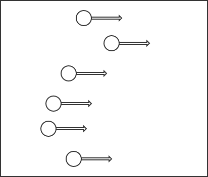
Fig. 20 An example of non ergodic system.

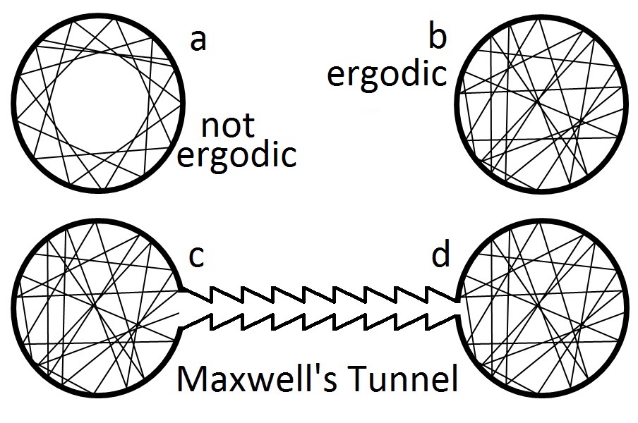
Another case from Wikipedia :

Pros

Poincaré recurrence theorem proves that at least some systems will come back to a state that is very close the the initial state after a long but finite time.
Systems are often chaotic so it’s not really possible to have pictures like the first one in Cons.

Poincare Recurrence Theorem

There is a very interesting paper regarding the recurrence theorem.

Dyson, F. J., & Falk, H. (1992). Period of a Discrete Cat Mapping. The American Mathematical Monthly, 99(7), 603.

The Liouville density evolution is written as

\[\frac{\partial}{\partial t} \rho = \{ H, \rho \},\]

while the von Neumann equation is

\[i\hbar \frac{\partial}{\partial t} \hat\rho = [\hat H, \hat\rho ].\]

The two equations are combined into one unified form

\[i \frac{\partial\rho}{\partial t} = \hat L \rho\]

where \(\hat L\) is the Liouville operator.

The thermodynamic observables are calculated using the probabilities of each state,

\[\avg{O} = \mathrm{Tr} \rho O\]

As long as \(\rho\) is not changed, the detailed dynamics and kinematics of the microscopic configurations doesn’t contribute the dynamics of the macroscopic observables.

Why does Ensemble Theory Work?

In principle, only one trace in phase space represents the actual kinematics of one lab system. Why is statistical sampling and statistical average working?

In ensemble theory, what we calculated is the ensemble average. Since we are dealing with equilibrium, we need the time average because we only have one lab system and the lab system evolve in time. Thus time average is the desired result. Since ensemble theory assume the replicas to be in equilibrium, each replica is serving as a snapshot of the system at different time. In this sense, ensemble average should be the same as time average.

Equilibrium¶

Equilibrium means that

\[\frac{\partial}{\partial} \rho = 0\]

or equivalently,

\[\{ H, \rho \} =0\]

Applying the knowledge of quantum mechanics, one possible solution is

\[\rho \propto e^{-\beta H}\]

The Three Most Used Ensembles¶

Table 1 Three Most Used Ensembles and Systems¶
Systems	Ensembles	Geometry in Phase space	Key Variables
Isolated	Microcanonical	Shell; \(\rho = c'\delta(E-H)\)	Energy \(E\)
Weak interacting	Canonical
Exchange particles	Grand canonical

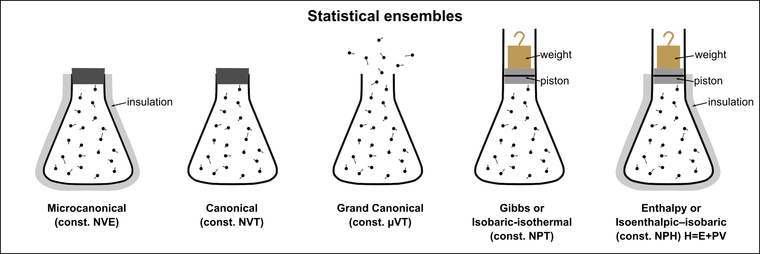
Fig. 21 Visual schematic representations of statistical ensembles. By Nzjacobmartin - Own work, CC BY-SA 4.0..

Isolated System - Micro-canonical Ensemble¶

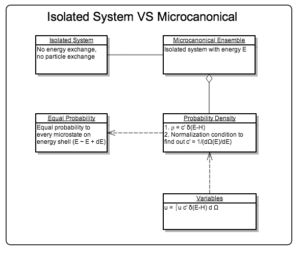
The system stays on the energy shell in phase space,

\[\rho(p;q;0) = \delta(H(p;q;0) - E)\]

The energy is also constant,

\[H(p;q;t) = E\]

For ergodic systems, ensemble average is equal to time average.

Important

What if the system stays longer in some regions on the phase sparce shell? How can we make sure the ensemble average is the same as time average?

Microcanonical ensembles are for isolated systems.

\[\rho \propto \frac{1}{\text{No. of states on the ensemble surface}} \equiv \frac{1}{\Omega (E)}\]

To calculate the entropy, the famous relation by Boltzmann is applied

\[S = k_B \ln \Omega\]

Canonical Ensemble¶

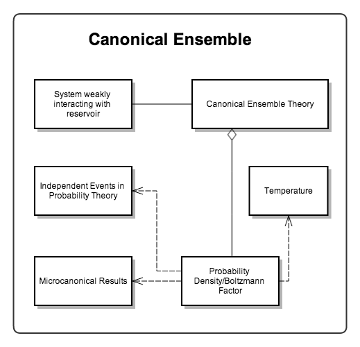
For a system weakly interacting with a heat bath, the total energy of the system is

\[E_T = E_S + E_R + E _{S,R}\]

where the interacting energy \(E_{S,R}\) is very small compared to the system energy, \(E_{S,R}\ll E_{S}\). We drop this interaction energy term, so that

\[E_T = E_S + E _R\]

A simple and intuitive derivation of the probability density is to use the theory of independent events.

\(\rho_T d\Omega_T\): probability of states in phase space volume \(d\Omega_T\);
\(\rho_S d \Omega_S\): probability of states in phase space volume \(d\Omega_S\);
\(\rho_R d \Omega_R\): probability of states in phase space volume \(d\Omega_R\);

We have assumed weak interactions between the system and the reservoir, so (approximately) the probability in the system phase space and in reservoir phase space are independent of each other,

\[\rho _ T d\Omega_T = \rho _S d\Omega_S \cdot \rho _R d \Omega_R .\]

Since there is no particle exchange between the two systems, overall phase space volume is the system phase space volume multiplied by reservoir phase space volume,

\[d\Omega_T = d\Omega _S \cdot d\Omega_R .\]

Obviously we can get the relationship between the three probability densities,

\[\rho_T = \rho_R \rho_S .\]

Take the logarithm of \(\rho_T\),

\[\ln\rho_T = \ln\rho_R + \ln\rho_S .\]

Key: \(\rho\) is a function of energy \(E\). AND both \(\rho\) and energy are extensive. The only possible form of \(\ln \rho\) is linear.

Finally we get,

\[\ln \rho = - \alpha - \beta E\]

i.e.,

\[\rho = e^{-\alpha} e^{-\beta E}\]

which is called canonical distribution.

Warning

This is not an rigorous derivation. Read RuKeng Su’s book for a more detailed and rigorous derivation.

Grand Canonical Ensemble¶

Systems with changing particle number are described by grand canonical ensemble.

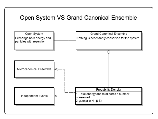
Here we only write donn the partition function of grand canonical ensemble

\[Z = \sum _ n \sum_N e^{-\beta E_n - \mu N} = \sum_N \left( \sum _ n e^{- \beta E _ n} \right)\left(e^{-\mu}\right)^N = \sum _ N Z \left(Z^f\right)^N\]

Identical Particles¶

If a system consists of \(N\) indentical particles, for any state \(n_i^\xi\) particles in particle state i, the energy of the system on state \(\xi\) is

\[E^\xi = \sum_i \epsilon_i n_i^\xi\]

where the summation is over all possible states of particles.

The energy is given by ensemble average

\[\avg{E} = \frac{\sum _\xi e^{-\beta E^\xi} E^\xi}{\sum _\xi e^{-\beta E^\xi}}\]

where \(\xi\) is the ensemble summation.

The Three Ensembles Continued¶

The three ensembles are the same when particle number N of the system becomes large enough, \(N\rightarrow 0\).

Here are the arguments:

When N is large enough, the interactions between the system and the reservoir are negligible. The extreme energies are rarely observed so that the distributions approach the Gaussian distribution. The variance of Gaussian distribution is proportional to \(1/\sqrt{N}\).
We have \(dE_S+dE_R=dE\) and \(dE=0\). When the energy of the system increases, that of the reservoir drops.

Most Probable Distribution¶

Boltzmann’s theory is about the most probable distribution of the single particle energy states.

For classical distinguishable particles, \(a_l = w_l e^{-\alpha -\beta e_l}\);
For bosons, \(a_l = w_l \frac{1}{e^{\alpha+\beta e_l} - 1}\);
For fermions, \(a_l = w_l \frac{1}{e^{\alpha + \beta e_l} + 1}\).

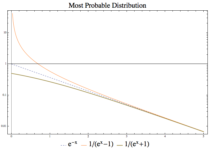
This figure shows that the three lines converge when the factor \(\alpha + \beta e_l\) is large enough. Fermions have less microstates than classical particles because of the Pauli exclusive principle.

\(\alpha + \beta e_l\) being large corresponds to several different physical meanings.

Temperature is low;
Energy is high;
Chemical coupling coefficient \(\alpha\) is large.

We have several identical conditions for the three distribution to be the same.

\[\alpha + \beta e_l \gg 1 \Leftrightarrow \alpha \gg 1 \Leftrightarrow 1/\exp(\alpha + \beta e_l) \ll 1 \Leftrightarrow a_l / w_l \ll 1\]

where the last statement is quite interesting. \(a_l/w_l \ll 1\) means we have much more states then particles and the quantum effects becomes very small.

Warning

One should be careful that even when the above conditions are satisfied, the number of micro states for classical particles is very different from quantum particles,

\[\Omega_{B.E} = \Omega_{F.D.} = \Omega_{M.B.}/N! .\]

This will have effects on entropy eventually.

Recall that thermal wavelength \(\lambda_t\) is a useful method of analyzing the quantum effect. At high temperature, thermal wavelength becomes small and the system is more classical.

Hint

Massive particles \(\lambda_t = \frac{h}{p} = \frac{h}{\sqrt{2m K}} = \frac{h}{\sqrt{ 2\pi m k T }}\)
Massless particles \(\lambda_t = \frac{c h}{2\pi^{1/3} k T}\)

However, at high temperature, the three micro states numbers are going to be very different. This is because thermal wavelength consider the movement of particles and high temperature means large momentum thus classical. The number of micro states comes from a discussion of occupation of states.

Important

What’s the difference between ensemble probability density and most probable distribution? What makes the +1 or -1 in the occupation number?

Most probable distribution is the method used in Boltzmann’s theory while ensemble probability density is in ensemble theory. That means in ensemble theory all copies (states) in a canonical ensemble appear with a probability density \(\exp(-\beta E)\) and all information about the type of particles is in Hamiltonian.

Being different from ensemble theory, Boltzmann’s theory deals with number of micro states which is affected by the type of particles. Suppose we have N particles in a system and occupying \(e_l\) energy levels with a number of \(a_l\) particles. Note that we have a degeneration of \(w_l\) on each energy levels.

(Gliffy source here .)

For Boltzmann’s theory, we need to

Calculate the number of micro states of the system;
Calculate most probable distribution using Lagrange multipliers;
Calculate the average of an observable using the most probable distribution.

Calculation of number of micro states

Calculation of the number of micro states requires some basic knowledge of different types of particles.

For classical particles, we can distinguish each particle from others and no restrictions on the number of states on each energy level. Now we have \(w_l^{a_l}\) possible states for each energy level. Since the particles are distinguishable we can have \(N!\) possible ways of exchanging particles. But the degenerated particles won’t contribute to the exchange (for they are the same and not distinguishable) which is calculated by \(\Pi_l a_l!\).

Finally we have

\[\Omega _{M.B.} = \frac{N!}{\Pi_l a_l !} \Pi_l w_l^{a_l}\]

as the number of possible states.

With similar techniques which is explicitly explained on Wang’s book, we get the number of micro states for the other two types of particles.

\[\Omega _{B.E.} = \Pi_l \frac{(a_l+w_l-1)}{a_l!(w_l -1)!}\]

is the number of micro states for a Boson system with a \(\{a_l\}\) distribution.

\[\Omega _ {F.D.} = \Pi _ {l} C_{w_l}^{a_l} = \Pi _ l \frac{w_l!}{a_l!(w_l - a_l)!}\]

is the number of micro states for a Fermion system with a distribution \(\{a_l\}\). We get this because we just need to pick out \(a_l\) states for \(a_l\) particles on the energy level.

The Exact Partition Function¶

DoS and partition function have already been discussed in previous notes.

Is There A Gap Between Fermion and Boson?¶

Suppose we know only M.B. distribution, by applying this to harmonic oscillators we can find that

\[\avg{H} = (\bar n + 1/2)\hbar \omega\]

where \(\bar n\) is given by

\[\bar n = \frac{1}{e^{\beta \hbar \omega} - 1}\]

which clearly indicates a new type of Boson particles.

So classical statistical mechanics and quantum statistical mechanics are closely connected not only in the most micro state numbers but also in a more fundamental way.

Hint

Note that this is possible because energy differences between energy levels are the same for arbitrary adjacent energy levels. Adding one new imagined particle with energy \(\hbar\omega\) is equivalence to excite one particle to higher energy levels. So we can treat the imagined particle as a Boson particle.