Important Questions of Statistical Mechanics¶

Liouville Operator And Liouville Equation¶

Instead of writing Poisson bracket as a bracket, Poisson bracket operator is defined to simplify the notation,

\[\hat{\mathscr H}^N = - \sum_{j=1}^N \left( \frac{\partial H^N}{\partial \vec q_j}\frac{\partial}{\partial \vec p_j} - \frac{\partial H^N}{\partial \vec p_j}\frac{\partial}{\partial \vec q_j} \right)\]

For convenience, we can define a Liouville operator,

\[\hat L^N := -i \hat{\mathscr H}^N .\]

so that the Liouville equation becomes

\[i \frac{\partial \rho^N}{\partial t} = \hat L^N \rho^N .\]

For stationary state, \(\frac{\partial \rho^N}{\partial t} = 0\), i.e.,

\[\hat L^N \rho^N _ {\mathrm{stationary}} = 0 .\]

BBGKY Hierarchy¶

To solve the statistical system completely, the most ideal method is to solve the Liouville equation directly, but without initial conditions given. However, solving the Liouville equation is impractical for complicated systems. Some simplifications have to be applied.

For systems without self-interactions, the solution of Liouville equation is straight forward. \(\Gamma\) space can actually be reduced to \(\mu\) space which is spanned by the freedoms of only one particle. Here we need to address the fact that we are dealing with identical particles.

We reduce the complicity of the interactions while keeping the salient features. Dimension reduction is key to this idea. First of all, we will introduce some reduced densities.

The probability density of particles describes the average density of some particles inside a system of particles.

For one particle, the probability density requires us to integrate over all other particles,

\[\rho_1(\vec X_1, t) := \int \cdots\int d\vec X_2 \cdots d \vec X_N \rho^N(\vec X_1, \cdots, \vec X_N, t)\]

Similarly, we can define \(s\) particles probability density, [Reichl]

\[\rho_s(\vec X_s, \cdots, \vec X_N, t) := \int \cdots \int d \vec X_{s+1}\cdots d\vec X_N \rho^N(\vec X_1, \cdots, \vec X_N, t) .\]

We define a normalized density

\[F_s(\vec X_1, \cdots,\vec X_s,t) := V^s \int\cdots \int \rho^N(\vec X_{1}, \cdots, \vec X_N, t) d\vec X_{s+1}\cdots d\vec X_N .\]

About \(V\)

Setting \(s=N\) leads to

\[F_N(t) = V^N \rho^N(t) .\]

We can write down the Hamiltonian of the system for any two-body spherically symmetric interaction,

\[H^N = \sum_{i=1}^N \frac{\vec p_i^2}{2m} + \sum_{i<j}^{N(N-1)/2} \phi(|\vec q_i - \vec q_j|) .\]

Recall that Liouville equation reads

\[\frac{\partial \rho^N}{\partial t} = - \hat L^N \rho^N .\]

Now we have

\[\hat{\mathscr H^N} = \sum_{i=1}^N \frac{\vec p_i}{m}\frac{\partial}{\partial \vec q_i} - \sum_{i<j}\hat \Theta_{ij}\]

where

\[\hat \Theta_{ij} := \frac{\partial \phi_{ij} }{\partial \vec q_i}\frac{\partial }{\partial \vec p_i} + \frac{\partial \phi_{ij}}{\partial \vec q_j} \frac{\partial}{\partial \vec p_j}\]

Write down the explicit Liouville equation for this problem and integrate over \(\{ \vec X_{s+1}, \cdots, \vec X_N \}\). Using approximation of large N limit, we derive a hierarchical set of equations,

\[\frac{\partial F_s}{\partial t} + \hat{\mathscr H^s} F_s = \frac{1}{v}\sum_{i=1}^s\int d\vec X_{s+1} \hat \Theta_{i,s+1} F_{s+1}(\vec X_1,\cdots,\vec X_{s+1}, t)\]

where \(v=V/N\).

The smaller \(s\) is, the lower the order of differentials is, thus the easier the solution seems to be. Unfortunately, to find out \(s=1\), we need \(s=2\) and the hierarchy goes haywire. Sooner or later, we have to cut the hierarchy manually.

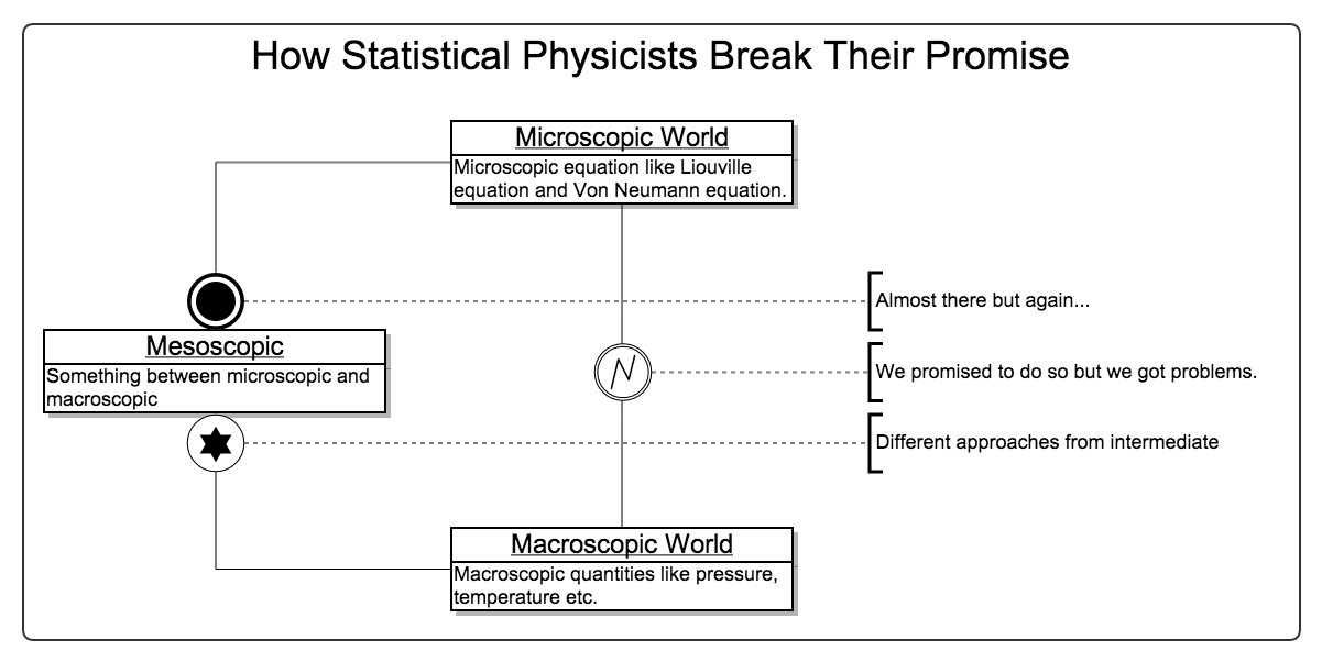
Road Map of Statistical Mechanics¶

As mentioned previously, the ideal situation is to solve Liouville equation directly and exactly. However, it’s generally impossible. The knowledge in between marcoscopic and microscopic, aka, mesoscropic, can help.

We start from the microscopic equations, then trucate at some hierarchy. Approximated results can be obtained. Then the approximated result is used to calculate the marcoscopic quantities.

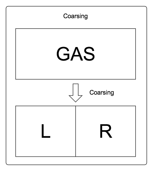
How Statistical Physicists Break Their Promise

We investigate a box of gas. First of all, we divide the box of gas into two parts. Two states, i.e., the LEFT state and the RIGHT state, are discussed instead of states in the whole phase space.

We can write down two equations using our intuition,

\[\frac{d P_L}{d t} = T_{LR} P_R - T_{RL}P_L\]

and

\[\frac{d P_R}{d t} = T_{RL} P_L - T_{LR}P_R .\]

The first equation means that the change of probability that a particle is in LEFT state is the rate from RIGHT to LEFT times the probability that the particle is in RIGHT state, minus the rate from LEFT state to RIGHT state times the probability that the particle is in LEFT state. This is just simply an linear model of gains and loses.

This is a coarse grained view. More generally, we have

\[\frac{d}{d t} P_\xi = \sum_\mu \left( T_{\xi\mu}P_\mu - T_{\mu\xi} P_{\xi} \right) .\]

The important thing is that these equations are linear.

Now we can start form these equations instead of the Liouville equation to solve the problem. It’s called mesoscopic. We simply need to connect these mesoscopic equations to the microscopic equations.

Why Irreversible¶

The reason that a system is irreversible is because we’ve lost information. In other words, the correlation function of time is short as the any system would be coupled to the reservoir. So any system would transfer information in and out into the reservoir and the information just dissipates deep into the reservoir. With information loss the system can not be reversible. In quantum mechanics, the system loses information (mostly) throught entanglement.

The classical idea of irreversibility is through H theorem. Boltzmann defined a \(H\) functional to measure the irreversibility

\[H = \int\int \rho(\vec r,\vec v, t) \ln \rho(\vec r,\vec v, t) d\tau d\omega\]

where \(d\tau d\omega\) is the infinitesemal volume in \(\mu\) space, \(\rho(\vec r,\vec v, t)\) is the probability density.

Boltzmann then proved that this \(H\) functional can not decrease for isolated and weakly interacting systems.

This result shows the statistical mechanics view of the second law of thermodynamics, which indicates that adiabatic process can never decrease the entropy of a system.

A Review of Boltzmann Equation & H Theorem¶

We will

Derive Boltzmann equation from classical scattering theory of rigid balls.
Derive continuity equation from Boltzmann equation.
Prove H theorem.
Understand H theorem.

Boltzmann equation derivation¶

The idea is to find an equation for one particle probability density \(f_j(\vec r, \vec v_j,t)\) by considering the number of particles move into this state and out of state due to collisions between the particles. Since we can find all contributions to \(f_j\) by applying scattering theory of classical particles, this equation can be written down explicitly. It will be an integrodifferential equation.

The number of particles in a differential volume \(d\vec r d\vec v\) at position \(\vec r\) with velocity \(\vec v_j\) is

\[f_j(\vec r, \vec v_j,t)d\vec r d\vec v_j .\]

Consider the distribution in a short time \(dt\). We write down the change of particle numbers due to collision and we find the Boltzmann equation.

\[\frac{\partial f_j}{\partial t} + \vec v_j\cdot \nabla _ {\vec r}f_j + \frac{\vec X _ j}{m_j} \cdot \nabla_{\vec v_j} f_j = 2\pi \sum_i \iint \left(f _ i'f _ j' - f _ i f _ j\right) g _ {ij} b \mathrm db \mathrm d \vec v_i\]

where \(\vec X\) is the external force on the particle, the prime \({}'\) denotes the quantity after collision, and \(b\) is the impact parameter.

Derivation

In the derivation, the most important part is to identify the number of particles into and out of this state due to collisions.

Boltzmann equation & Continuity Equation¶

We can derive from the Boltzmann equation the Enskog’s equation and continuity equation by choosing an conserved quantity as \(\psi_i\) in Enskog’s equation.

H Theorem¶

H theorem says that the functional \(H\) can not decrease. This particular derivation requires a classical, particle number conserved system.

Define the \(H\) functional,

\[H(t) = \iint f(\vec r, \vec v, t) \ln f(\vec r, \vec v, t) d\vec r d\vec v\]

Using the Boltzmann equation derived previously, the following relation is proved

\[\frac{d H}{dt} \leq 0\]

in which equal sign is valid if&f

\[f' f_1' = f f_1 .\]

H Theorem Discussions¶

There were two objections on H theorem:

Loschmidt: All collisions can be reversed in the view of classical mechanics;
Zermelo: Poincare recursion theorem says an equilibrium system can go back to inequilibrium.

To Loschmidt’s questioning, Boltzmann pointed out that H theorem is a statistical theorem rather than mechanics theorem. Quantities in this theorem like \(f\) are statistical averages, not the quantity of a specific particle.

Zermelo’s objection is not a serious problem because the recursion time is extremely long.

Footnotes¶

[Reichl]

1. Reichl, A Modern Course in Statistical Physics